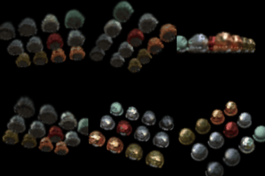
Pixels span [-1, 1]. Rays start at the camera center and point toward unprojected image-plane points. Rendering sums color and depth with alpha-transmittance weights.



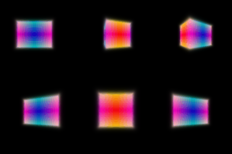
Center: (0.25, 0.25, 0.00). Side lengths: (2.01, 1.50, 1.50). Adam, learning rate 0.0005, 1,000 epochs, RGB mean squared error. The fitted box matches the target position and dimensions.
Six 128-unit layers with a skip connection, six position-encoding frequencies, ReLU density, and sigmoid RGB. Trained for 250 epochs on 128 × 128 Lego images, using 1,024 rays and 128 samples per ray.

| Experiment | PSNR (dB) | SSIM |
|---|---|---|
| Lego, validation views | 29.44 | 0.942 |
Direction encoding (two frequencies) enters only the color branch. Both materials models use 150 epochs, 512 rays, 64 samples, and learning rate 0.0001.
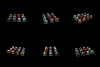
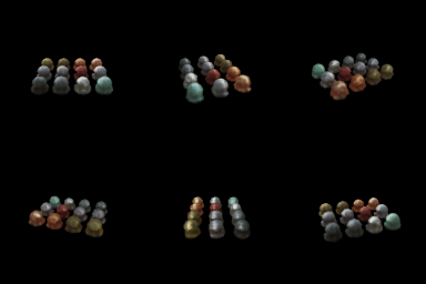
View-independent materials, followed by view-dependent materials:
| Experiment | PSNR (dB) | SSIM |
|---|---|---|
| View independent, validation | 25.08 | 0.864 |
| View dependent, validation | 25.73 | 0.871 |
Adding viewing direction increased validation PSNR by 0.66 dB in this run. View dependence can represent changing highlights. Greater directional capacity can memorize training views; keeping direction out of density and using a small color branch limits that risk.
The coarse network evaluates 64 uniform samples. Its detached weights define a PDF for 64 additional samples; a separate fine network evaluates the 128 sorted samples. Both color losses train the networks. NeRF paper.

| Experiment | PSNR (dB) | SSIM |
|---|---|---|
| Uniform (250 epochs, 1,024 rays) | 29.44 | 0.942 |
| Coarse/fine (150 epochs, 512 rays) | 28.68 | 0.932 |
Median GPU time on the A10G for 1,024 rays (20 forwards after five warm-ups): uniform 5.77 ms; coarse/fine 8.77 ms. Importance sampling concentrates work near visible surfaces, but adds a network pass and can miss features absent from the coarse PDF. These quality results use different training budgets, so they do not isolate the effect of sampling.
A positional MLP predicts a signed-distance residual to an initial sphere; a second MLP predicts color. The Eikonal loss penalizes (|gradient SDF| − 1)². VolSDF paper.
| Experiment | PSNR (dB) | SSIM |
|---|---|---|
| Beta 0.05, 250 epochs | 24.40 | 0.859 |
| Beta 0.02, 50 further epochs | 24.81 | 0.882 |
Alpha is 10, the Eikonal weight is 0.02, the initial learning rate is 0.0005, and there are 128 samples per ray. Alpha keeps interiors opaque while the Eikonal penalty regularizes distance gradients. The lower-beta run continues the default run; it is a refinement experiment rather than a controlled beta-only comparison. The displayed model is the lower-beta refinement, selected by validation PSNR.
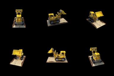
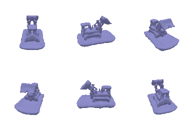
Alpha and beta: Alpha scales density and opacity; beta controls the thickness of the transition around the zero-level surface.
High versus low beta: High beta spreads density across a wider region and favors smoother, less precise boundaries. Low beta concentrates density near the surface and permits sharper boundaries.
Easier to train: High beta usually gives useful gradients over a wider region, making coarse sampling and early optimization more forgiving.
More accurate surface: Low beta can give a tighter correspondence between rendered boundaries and the SDF surface, provided sampling resolves the thin transition.
All four supplied Gaussian unit tests pass. The renderer projects covariances, filters and sorts by depth, and blends RGB, depth, and silhouette with front-to-back transmittance. 3D Gaussian Splatting paper. Chair rendering resolution: 128 × 128; displayed panels are enlarged to 256 × 256.

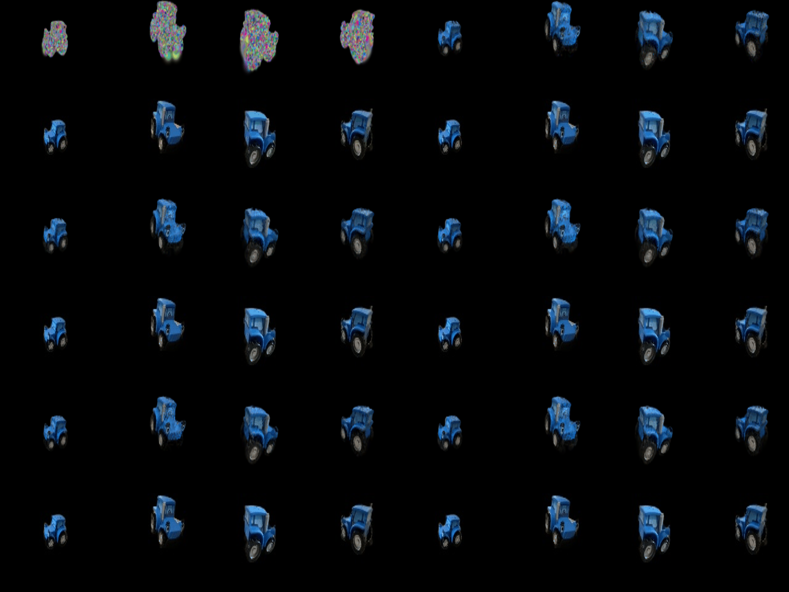
Truck: 10,000 isotropic Gaussians initialized from the provided points, Adam, L1 loss, 1,000 iterations. Learning rates: means 0.0002; scales 0.005; colors 0.01; opacities 0.05. Rotations are fixed for isotropic Gaussians.
| Experiment | PSNR (dB) | SSIM |
|---|---|---|
| Truck, held-out test views | 29.50 | 0.939 |

All 16 real spherical-harmonic basis functions through degree three modulate RGB using normalized camera-to-Gaussian directions. SH coefficient convention.
Without spherical harmonics:
With spherical harmonics:

Left: DC only. Right: spherical harmonics. Each pair uses exactly the same camera.

Frame 8: spherical harmonics darken the seat upholstery and increase its contrast.

Frame 16: the seat becomes darker, making its worn patches more distinct.

Frame 24: the back view changes less, with only subtle upholstery-color changes. Geometry stays unchanged.
Baseline: 10,000 randomly initialized isotropic Gaussians, the same learning rates and L1 loss as the truck, and 1,000 iterations.
Improved: 10,000 anisotropic Gaussians initialized uniformly in [-1.2, 1.2]³, initial scale 0.025, and initial opacity sigmoid(-2.2). Mean learning rate starts at 0.001; other rates match the baseline, with rotation rate 0.001. All rates decay exponentially to one tenth over 3,000 iterations. L1 loss is unchanged.
| Experiment | PSNR (dB) | SSIM |
|---|---|---|
| Materials baseline, validation | 19.24 | 0.681 |
| Materials improved, validation | 26.18 | 0.893 |
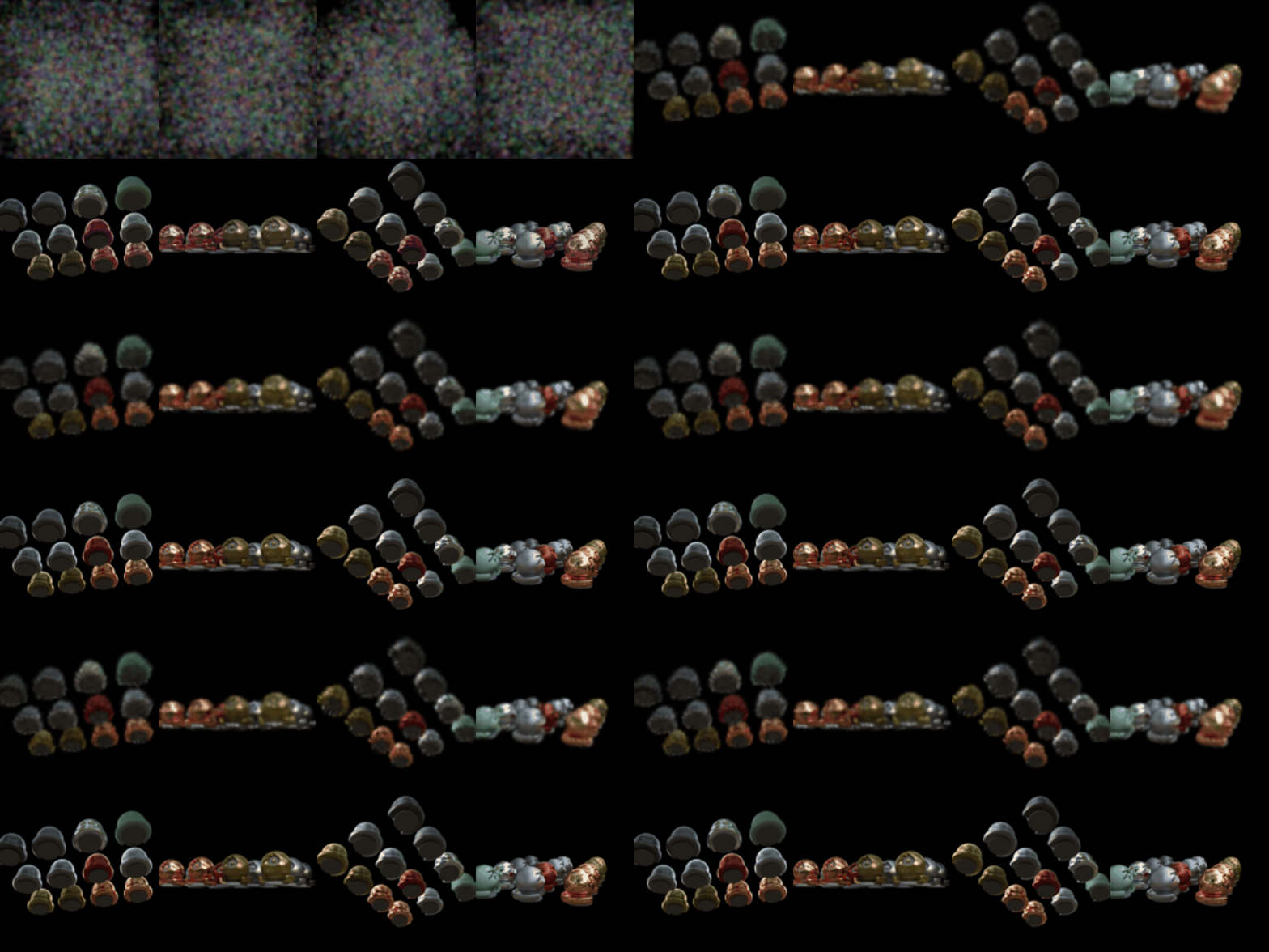
The improved setup increased validation PSNR by 6.94 dB. The baseline forms central blobs; the improved model recovers separated objects, although highlights remain soft. Wider initialization covers the separated objects; lower opacity reduces early occlusion. Anisotropic scales fit directional structure, while the longer run and learning-rate decay allow finer adjustment.
Baseline progress and final views:
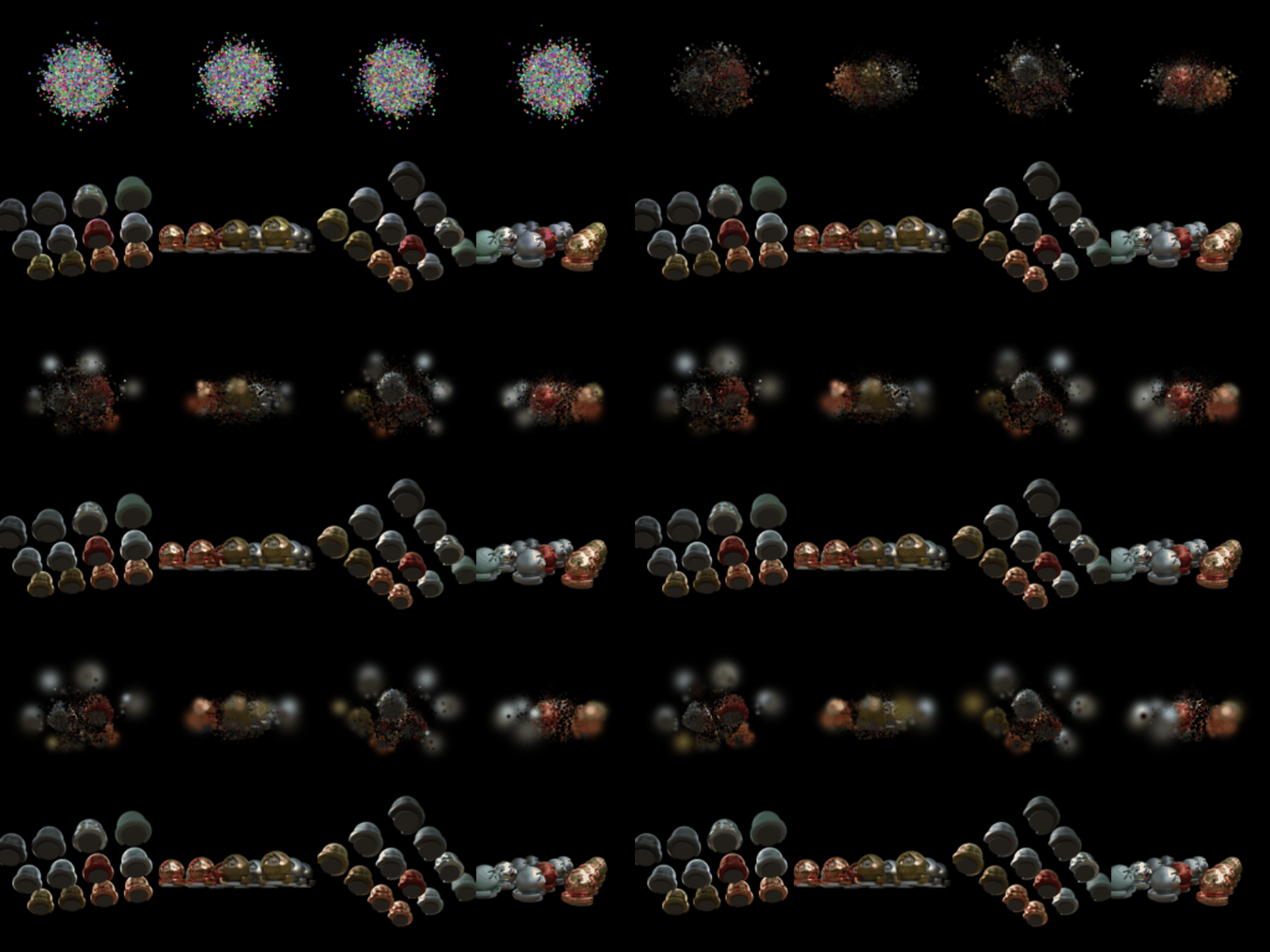

Improved progress and final views: