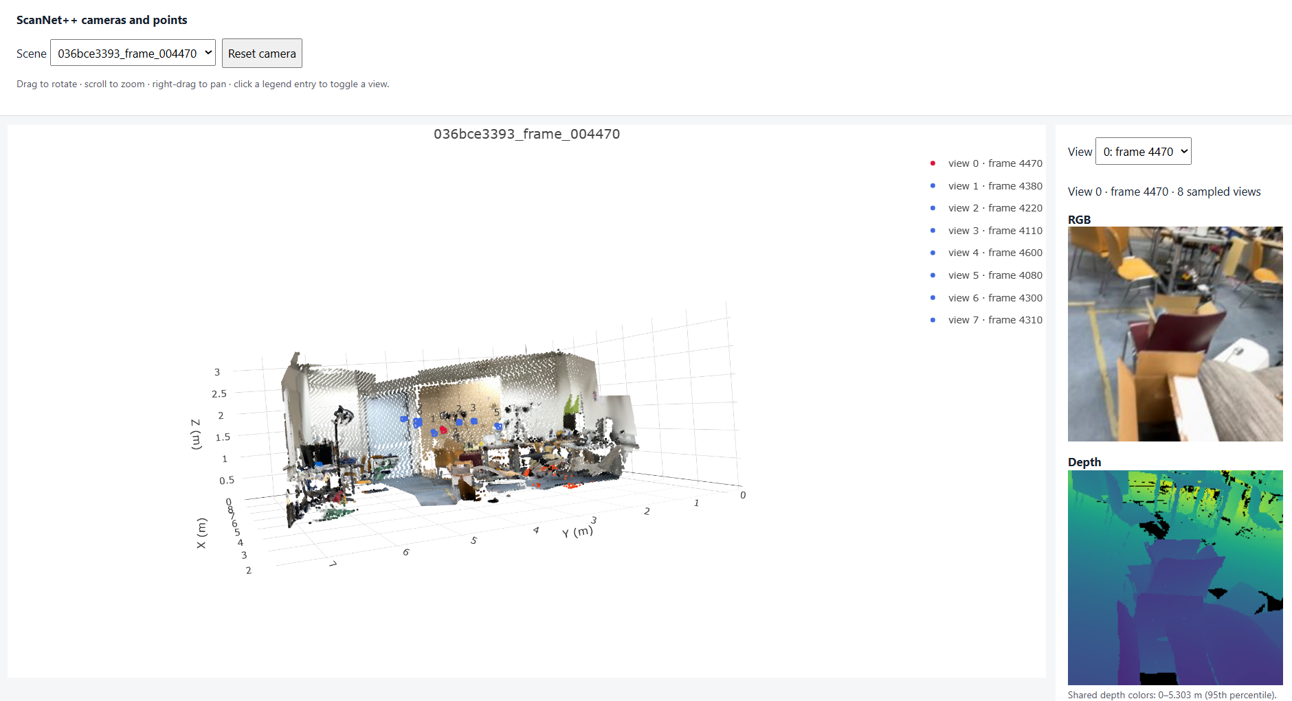
Scene 1: points and cameras in the original world frame (meters)
Name: Yuqin Jiao | Andrew ID: sjiao2
After resizing the intrinsics (Q1.1) and unprojecting optical-axis z-depth (Q1.2), 3D points and cameras are still in the original ScanNet++ world frame, in meters. Different scenes have different origins, orientations and metric scales.
Scene 1: points and cameras in the original world frame (meters)
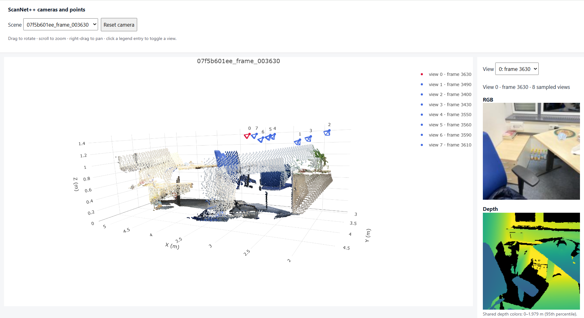
Scene 2: points and cameras in the original world frame (meters)
After Q1.3, camera 0 is the identity: its center is at the origin. Depth, points and the other poses are expressed in this frame and divided by the same scene scale, so the valid-point centroid is about 1 unit from the origin. The overlay on each screenshot reports the first camera center and the valid-point centroid distance.
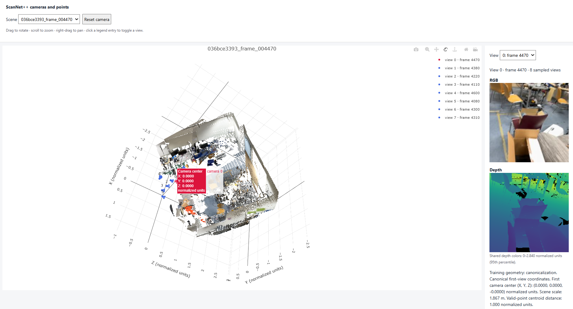
Scene 1: canonicalized geometry. First camera center ≈ (0, 0, 0); valid-point centroid distance ≈ 1.
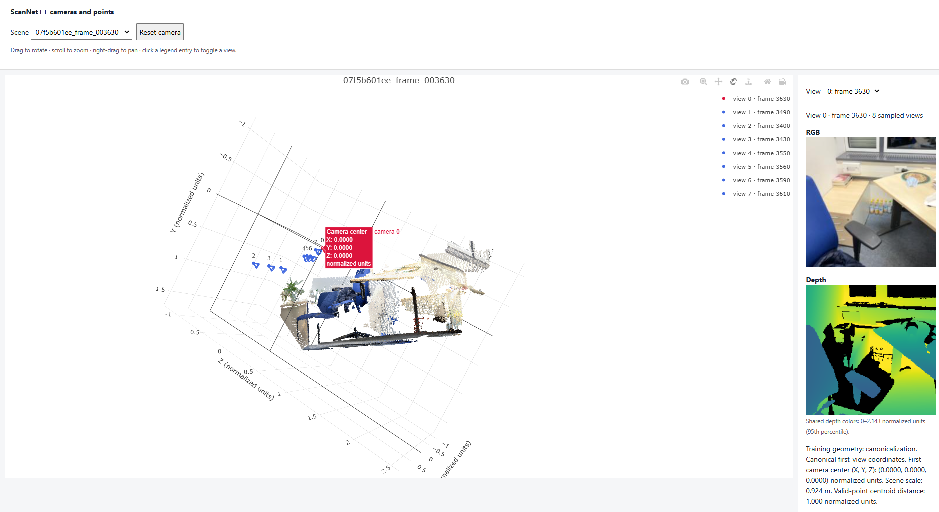
Scene 2: canonicalized geometry. First camera center ≈ (0, 0, 0); valid-point centroid distance ≈ 1.
Command: python scripts/check_data.py --config configs/scannetpp/iphone/data.json --split train --max-samples 4
All four samples pass the requested checks. Batch shapes match the data contract (8 views, 224×224, Plücker 6 channels). Point and ray reprojection errors are about 10−4 px, well below the 0.01 px threshold. The valid-point centroid distance is 1.0. Valid-depth fractions are high (0.75–0.99); the lower value is expected, because missing depth is stored as zero and is not used as geometry.
{
  "split": "train",
  "dataset_samples": 224,
  "checked_samples": 4,
  "samples": [
    {
      "sequence_name": "e050c15a8d_frame_007080",
      "views": 8,
      "resolution": 224,
      "valid_depth_fraction": 0.9779127240180969,
      "max_reprojection_error_px": 0.00011279189493507147,
      "max_ray_reprojection_error_px": 0.00010904046939685941,
      "centroid_distance": 1.0
    },
    {
      "sequence_name": "5f99900f09_frame_002820",
      "views": 8,
      "resolution": 224,
      "valid_depth_fraction": 0.9903116226196289,
      "max_reprojection_error_px": 0.00012302029062993824,
      "max_ray_reprojection_error_px": 0.00011108566104667261,
      "centroid_distance": 0.9999999403953552
    },
    {
      "sequence_name": "47b37eb6f9_frame_002720",
      "views": 8,
      "resolution": 224,
      "valid_depth_fraction": 0.9609947800636292,
      "max_reprojection_error_px": 9.881925507215783e-05,
      "max_ray_reprojection_error_px": 8.897326188161969e-05,
      "centroid_distance": 1.0
    },
    {
      "sequence_name": "4c5c60fa76_frame_006690",
      "views": 8,
      "resolution": 224,
      "valid_depth_fraction": 0.7516716122627258,
      "max_reprojection_error_px": 0.0001155954014393501,
      "max_ray_reprojection_error_px": 0.000106735089502763,
      "centroid_distance": 1.0
    }
  ],
  "batch_shapes": {
    "rgb": [2, 8, 3, 224, 224],
    "depth": [2, 8, 1, 224, 224],
    "depth_valid": [2, 8, 1, 224, 224],
    "K": [2, 8, 3, 3],
    "frame_numbers": [2, 8],
    "T_world_from_camera": [2, 8, 4, 4],
    "original_world_from_reference": [2, 4, 4],
    "scene_scale": [2],
    "points_world": [2, 8, 3, 224, 224],
    "ray_origins": [2, 8, 3, 224, 224],
    "ray_directions": [2, 8, 3, 224, 224],
    "plucker": [2, 8, 6, 224, 224]
  }
}
Canonicalization. Each sample is expressed in the first camera’s frame and divided by a shared scene scale (distance from that camera to the valid-point centroid). Camera 0 is identity, and the valid-point centroid has distance 1 from the origin. The centroid is not subtracted, so camera 0 stays at the origin.
World-space ray directions. For each pixel, the resized K maps the pixel to a camera-frame direction. The camera-to-world rotation takes it into the canonical world frame, then it is normalized to unit length. The ray origin is the camera center in that same frame.
Plücker moment. Each ray is six channels [d, m]: unit direction followed by moment, with m = o × d. Shifting the origin along the ray does not change m, so this encoding is the line itself, not a choice of starting point.
Command: python -m models.lvsm.train --overfit 2000 --output-dir outputs/lvsm_overfit
After 2000 steps on one fixed batch, the loss decreases steadily and the final overfit PSNR is 30.94 dB (target: ≥ 30 dB), confirming that patchify/unpatchify, token assembly and the loss are implemented correctly.

val_epoch000.png after overfitting (columns: source views, ground truth, prediction)
Training settings.
configs/lvsm.json, command python -m models.lvsm.train --config configs/lvsm.jsonTraining curves.

Train / val MSE loss

Train / val PSNR
Validation metrics (best.pt).
Command: python -m models.lvsm.eval --checkpoint outputs/lvsm/best.pt --num-source-views 1 2 4 --conditioning correct shuffled none
| Source views | correct | shuffled | none | |||
|---|---|---|---|---|---|---|
| PSNR ↑ | SSIM ↑ | PSNR ↑ | SSIM ↑ | PSNR ↑ | SSIM ↑ | |
| 1 | 15.20 | 0.5584 | 11.81 | 0.4879 | 12.46 | 0.5301 |
| 2 | 16.15 | 0.5603 | 11.49 | 0.4721 | 12.43 | 0.5283 |
| 4 | 16.86 | 0.5753 | 11.60 | 0.4738 | 12.46 | 0.5379 |
Training visualization.

val_epoch095.png during training (columns: source views, ground truth, prediction)
Evaluation visualizations (correct conditioning).

1 source view
2 source views

4 source views
Evaluation visualizations (ray-conditioning ablation, 4 source views).

shuffled target rays
no target rays (all zeros)
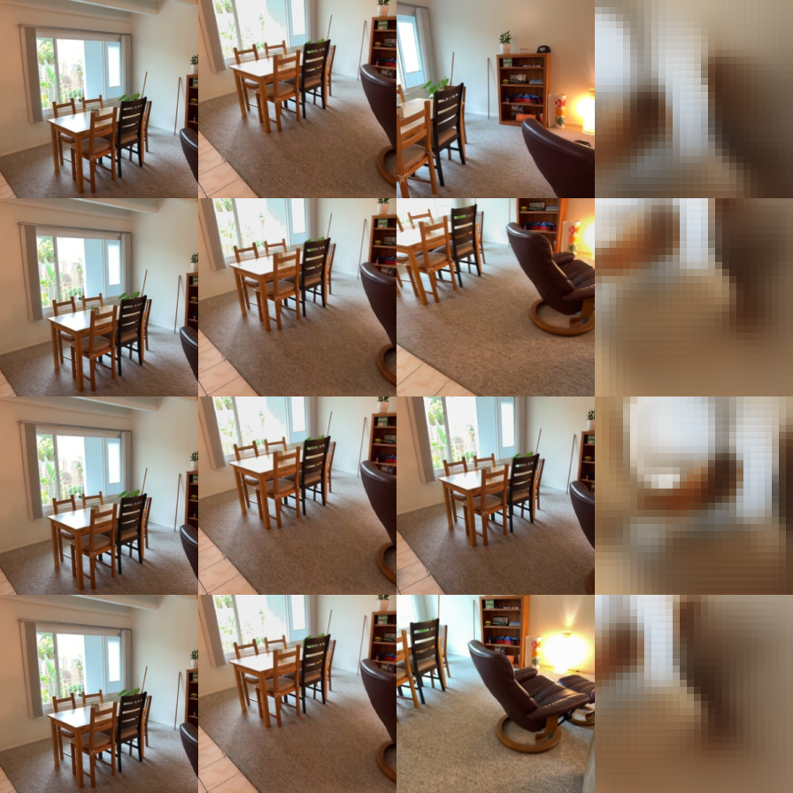
Effect of the number of source views. With correct rays, PSNR rises from 15.20 dB (1 view) to 16.15 dB (2 views) and 16.86 dB (4 views); SSIM follows (0.5584 → 0.5603 → 0.5753). Extra sources give more coverage of the target view, so the model has to invent fewer pixels. The gain is modest (+1.66 dB from 1 to 4 views).
Effect of ray conditioning. Target rays are what specify which view to render. Shuffled swaps in another target’s rays, and PSNR falls to 11.49–11.81 dB. None zeros the rays, and PSNR is 12.43–12.46 dB at every source count. Shuffled is worse than none: a wrong pose is more harmful than no pose. Adding source views does not help shuffled or none, so the bottleneck is the target camera, not missing source images. The gap from correct (16.86 dB) to shuffled / none (11.60 / 12.46 dB at 4 views) shows the model uses the Plücker rays rather than copying sources.
Question. How does training Mini-LVSM with only 1 source view change its evaluation performance with 1, 2 and 4 source views, compared with the baseline trained with 2 source views?
Experimental settings.
Everything is identical to the Q2.2 baseline (data, model size, learning rate, schedule, 100 epochs,
seed) except num_source_views = 1 in a copied config
configs/lvsm_views1.json (the baseline config was not modified).
Both models are evaluated on the validation split with
--num-source-views 1 2 4 --conditioning correct.
| Training source views | Eval 1 view | Eval 2 views | Eval 4 views | |||
|---|---|---|---|---|---|---|
| PSNR ↑ | SSIM ↑ | PSNR ↑ | SSIM ↑ | PSNR ↑ | SSIM ↑ | |
| 2 (baseline) | 15.20 | 0.5584 | 16.15 | 0.5603 | 16.86 | 0.5753 |
| 1 | 15.11 | 0.5591 | 14.91 | 0.5526 | 14.65 | 0.5612 |

Validation PSNR during training: baseline vs 1-view training

1-view-trained model, evaluated with 1 source view

1-view-trained model, evaluated with 4 source views
Results and discussion. At 1 source view the two models are tied: 15.11 dB (train S=1) vs 15.20 dB (baseline). Matching the train-time view count to this test setting does not improve single-view PSNR. Extra views then split them. From 1 to 4 views, the 1-view model drops 0.46 dB (15.11 → 14.65), while the baseline rises 1.66 dB (15.20 → 16.86). The 1-view model never saw more than one source during training, so it cannot use additional sources at test time.
Conclusion. Train-time source count controls which test counts work. Training with 1 view does not hurt 1-view evaluation, but extra views at test time do not help. Training with 2 views transfers to 1, 2 and 4 views, and PSNR increases with more sources.
Limitations. Each setting was trained once, so 15.11 vs 15.20 dB may be run-to-run noise. The 1-view model also has fewer source tokens per step, so compute is not matched to the baseline.
Command: python -m models.vggt.train --config configs/vggt.json --overfit --output outputs/vggt_overfit
40 epochs on one fixed training clip (25 steps/epoch, lr 1e-3). Loss decreases steadily, and after overfitting the clip has
AbsRel 0.037, δ1 0.955, rotation error 0.16° and translation-direction error 0.45°.
Depth loss becomes negative because the confidence term contains -0.2 log(conf).

Overfit loss curve (total, camera and depth). Final train loss −0.161 (camera 0.0025, depth −0.174).
Predicted cameras and the reconstructed point cloud close to GT on clip 036bce3393_frame_004470.

GT geometry

Predicted geometry
Training settings.
configs/vggt.json, command python -m models.vggt.train --config configs/vggt.json --output outputs/vggt_trainTraining curves.

Train / val total, camera and depth loss
Validation / test metrics (best.pt).
Command: python -m models.vggt.eval --checkpoint outputs/vggt_train/best.pt --split {val,test} --eval-root data/scannetpp/prepared_eval --num-views 8 --eval-num-frames 32 --image-size 224 --seed 825
| Metric | Val | Test |
|---|---|---|
| Depth AbsRel ↓ | 0.128 | 0.151 |
| Depth δ1 ↑ | 0.866 | 0.805 |
| Rotation AUC@5° ↑ | 0.183 | 0.203 |
| Rotation AUC@15° ↑ | 0.520 | 0.535 |
| Rotation AUC@30° ↑ | 0.713 | 0.724 |
| Translation AUC@5° ↑ | 0.009 | 0.014 |
| Translation AUC@15° ↑ | 0.083 | 0.077 |
| Translation AUC@30° ↑ | 0.201 | 0.189 |
| Joint Pose AUC@5° ↑ | 0.003 | 0.005 |
| Joint Pose AUC@15° ↑ | 0.068 | 0.057 |
| Joint Pose AUC@30° ↑ | 0.185 | 0.169 |
GT vs. predicted geometry on four validation scenes.
From outputs/vggt_train/visualization/index.html, same camera angle for GT and Pred in each pair.

09c1414f1b GT

09c1414f1b Pred

21d970d8de GT

21d970d8de Pred

280b83fcf3 GT

280b83fcf3 Pred

2b1dc6d6a5 GT

2b1dc6d6a5 Pred
Errors on held-out scenes. Depth transfers better than pose: test AbsRel 0.151 vs val 0.128, δ1 0.805 vs 0.866. Rotation AUC (val 0.183 / 0.520 / 0.713) is much higher than translation AUC (0.009 / 0.083 / 0.201) at every threshold. AUC@5° is far below AUC@30°, so the pose is coarsely right but not precise; the camera head predicts once, without iterative refinement. The val/test gap is small and mixed (test rotation is slightly higher, translation is similar), which suggests systematic pose error rather than overfitting to the validation scenes.
Question. How does training Mini-VGGT with 4 input views instead of 8 change depth and pose accuracy, runtime and memory?
Experimental settings.
Everything is identical to the Q3.2 baseline (data, model, learning rate, schedule, 1000 epochs, seed, batch size 16,
sampling_range 32, camera/depth weights 5.0/1.0, one A100 40GB) except num_views = 4 in a copied config
configs/vggt_views4.json.
Each model is evaluated on its training view count with
--eval-num-frames 32 --image-size 224 --seed 825.
| Train / eval views | Depth | Rotation AUC ↑ | Translation AUC ↑ | Joint Pose AUC ↑ | |||||||
|---|---|---|---|---|---|---|---|---|---|---|---|
| AbsRel ↓ | δ1 ↑ | 5° | 15° | 30° | 5° | 15° | 30° | 5° | 15° | 30° | |
| 8, val | 0.128 | 0.866 | 0.183 | 0.520 | 0.713 | 0.009 | 0.083 | 0.201 | 0.003 | 0.068 | 0.185 |
| 4, val | 0.129 | 0.863 | 0.177 | 0.505 | 0.679 | 0.008 | 0.090 | 0.198 | 0.000 | 0.070 | 0.165 |
| 8, test | 0.151 | 0.805 | 0.203 | 0.535 | 0.724 | 0.014 | 0.077 | 0.189 | 0.005 | 0.057 | 0.169 |
| 4, test | 0.140 | 0.826 | 0.220 | 0.549 | 0.734 | 0.006 | 0.032 | 0.125 | 0.006 | 0.027 | 0.114 |
| Train views | Peak train memory | Wall-clock | Time / epoch |
|---|---|---|---|
| 8 | ≈ 15.5 GB | ≈ 5.5 h | ≈ 14 s |
| 4 | ≈ 8.3 GB | ≈ 3.8 h | ≈ 7 s |
Loss curve, 8-view training (Q3.2 baseline)

Loss curve, 4-view training

8-view model, 09c1414f1b_frame_000000

4-view model, same scene
Results and discussion. Halving the views cut peak memory from about 15.5 GB to 8.3 GB and time per epoch from about 14 s to 7 s (wall-clock 5.5 h → 3.8 h). Depth barely changes (val AbsRel 0.128 → 0.129, δ1 0.866 → 0.863; test AbsRel 0.140 vs 0.151). Pose is more sensitive: val rotation AUC@30° 0.713 → 0.679 and joint AUC@30° 0.185 → 0.165; on test, translation AUC@30° falls 0.189 → 0.125 and joint AUC@30° 0.169 → 0.114. 4 views give C(4,2)=6 pose pairs per sample instead of C(8,2)=28, so there is less multi-view evidence for translation.
Conclusion. 4 views save about 7 GB of memory and half the per-epoch time, with almost no depth drop. The cost is translation accuracy, especially on test. Use 4 views if the goal is depth under a memory limit; keep 8 views if pose matters.
Limitations. sampling_range was 32 in both runs, so view count and view density change together. The 4-view pose metrics average over fewer pairs (168 vs 784) and are noisier. Each setting was trained once, and each model was evaluated only at its training view count.