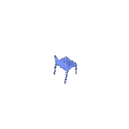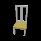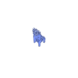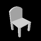
Assignment 2: Single View to 3D

Name: Yuqin Jiao  |  Andrew ID: sjiao2

1. Exploring loss functions (10 points)

1.1. Fitting a voxel grid (4 points)

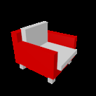
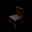
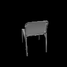
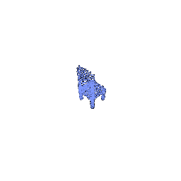
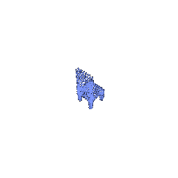
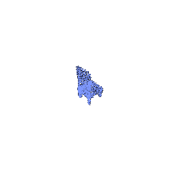
Visualize the optimized voxel grid along-side the ground truth voxel grid using the tools learnt in previous section.
Optimized voxel grid

Optimized voxel grid

Ground truth voxel grid
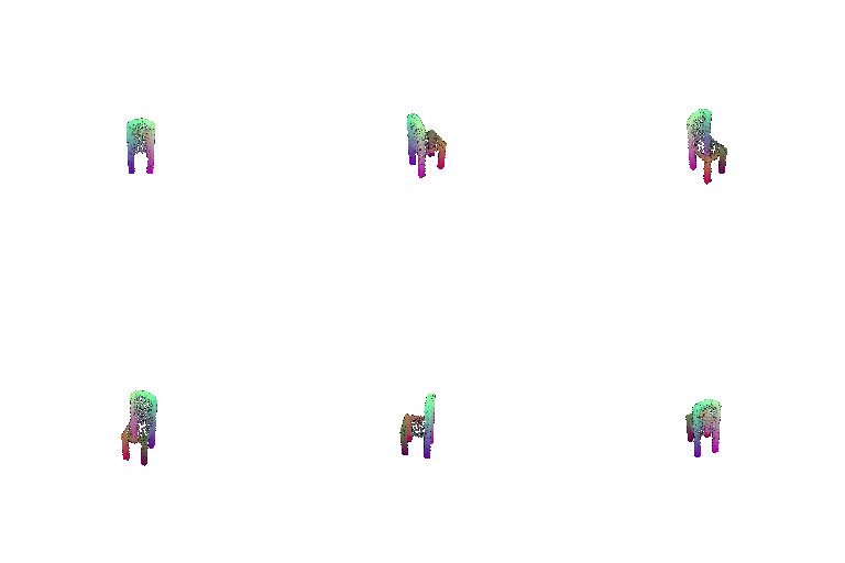
Ground truth voxel grid

1.2. Fitting a point cloud (3 points)

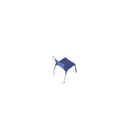
Visualize the optimized point cloud along-side the ground truth point cloud using the tools learnt in previous section.
Optimized point cloud

Optimized point cloud

Ground truth point cloud
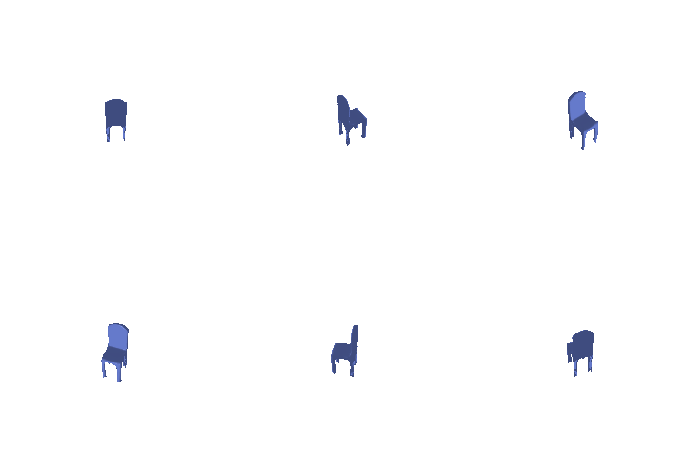
Ground truth point cloud

1.3. Fitting a mesh (3 points)

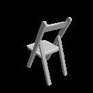
Visualize the optimized mesh along-side the ground truth mesh using the tools learnt in previous section.
Optimized mesh

Optimized mesh

Ground truth mesh

Ground truth mesh

2. Reconstructing 3D from single view (80 points)

You can also enable training on a CPU by the device argument. Also indiciate in your submission if you had to use this argument.

I used --load_feat for question 2.4, 2.5, 3.3.

2.1. Image to voxel grid (20 points)

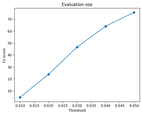
On your webpage, you should include visuals of any three examples in the test set. For each example show the input RGB, render of the predicted 3D voxel grid and a render of the ground truth mesh. Also report the F1@0.05 score and include the F1 plot, which is saved as eval_vox.png.

Example 1

vox example 1: input RGB

Input RGB

vox example 1: Predicted voxel grid

Predicted voxel grid

vox example 1: ground truth mesh

Ground truth

Example 2

vox example 2: input RGB

Input RGB

vox example 2: Predicted voxel grid

Predicted voxel grid

vox example 2: ground truth mesh

Ground truth

Example 3

vox example 3: input RGB

Input RGB

vox example 3: Predicted voxel grid

Predicted voxel grid

vox example 3: ground truth mesh

Ground truth

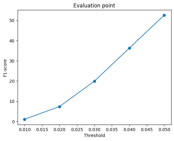
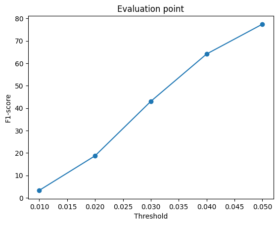
F1@0.05 score: 75.651

F1 plot for voxel grid (eval_vox.png)

2.2. Image to point cloud (20 points)

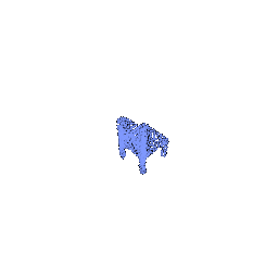
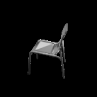
On your webpage, you should include visuals of any three examples in the test set. For each example show the input RGB, render of the predicted 3D point cloud and a render of the ground truth mesh. Also report the F1@0.05 score and include the F1 plot, which is saved as eval_point.png.

Example 1

point example 1: input RGB

Input RGB

point example 1: Predicted point cloud

Predicted point cloud

point example 1: ground truth mesh

Ground truth

Example 2

point example 2: input RGB

Input RGB

point example 2: Predicted point cloud

Predicted point cloud

point example 2: ground truth mesh

Ground truth

Example 3

point example 3: input RGB

Input RGB

point example 3: Predicted point cloud

Predicted point cloud

point example 3: ground truth mesh

Ground truth

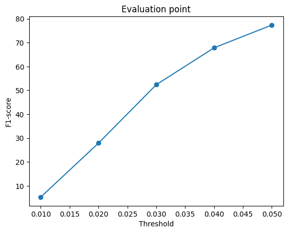
F1@0.05 score: 77.362

F1 plot for point cloud (eval_point.png)

2.3. Image to mesh (20 points)

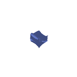
On your webpage, you should include visuals of any three examples in the test set. For each example show the input RGB, render of the predicted mesh and a render of the ground truth mesh. Also report the F1@0.05 score and include the F1 plot, which is saved as eval_mesh.png. Additionally, quantitatively compare the F1 score of 3D reconstruction for meshes vs pointcloud vs voxel grids. Provide an intuitive explaination justifying the comparision.

Example 1

mesh example 1: input RGB

Input RGB

mesh example 1: Predicted mesh

Predicted mesh

mesh example 1: ground truth mesh

Ground truth

Example 2

mesh example 2: input RGB

Input RGB

mesh example 2: Predicted mesh

Predicted mesh

mesh example 2: ground truth mesh

Ground truth

Example 3

mesh example 3: input RGB

Input RGB

mesh example 3: Predicted mesh

Predicted mesh

mesh example 3: ground truth mesh

Ground truth

F1@0.05 score: 73.204
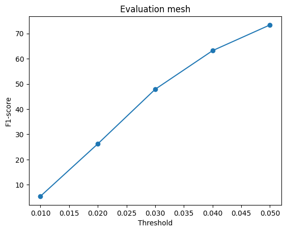
F1 plot for mesh (eval_mesh.png)

Quantitative comparison (F1@0.05):

RepresentationF1@0.05
Voxel grid75.651
Point cloud77.362
Mesh73.204

Intuitive explanation justifying the comparison: the mesh representation has the best visualization, but the point cloud representation shows the open part of chair better. The point cloud model has the highest F1@0.05 (77.362), followed by the voxel grid and the mesh, trained for 52, 74 and 98 iterations respectively. The mesh topology is usually better. The point cloud has no grid or fixed topology, so is more sparse.

2.4. Analyse effects of hyperparams variations (10 points)

Analyse the results, by varying a hyperparameter of your choice. For example n_points or vox_size or w_chamfer or initial mesh (ico_sphere) etc. Try to be unique and conclusive in your analysis.

Hyperparameter: n_points

I trained two point cloud models that differ only in n_points (100 and 1000), both for 4000 iterations, using--load_feat on the chair dataset. Both models are evaluated on the same chair set.

n_pointsF1@0.05
10052.565
100077.418

F1 plots:

F1 plot, n_points = 100

n_points = 100

F1 plot, n_points = 1000

n_points = 1000

Visual comparison (same test example):
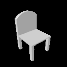
Input RGB

Input RGB

Prediction, n_points = 100

Prediction (n_points = 100)

Prediction, n_points = 1000

Prediction (n_points = 1000)

Analysis:

Increasing n_points from 100 to 1000 improves F1@0.05 from 52.565 to 77.418. For the samples, with 100 points the prediction is sparse and scattered, and the chair shape is not really recognizable, while with 1000 points the points are more concentrated and the prediction clearly looks like a chair. In this experiment, more points cover the chair surface more densely and give better results both quantitatively and visually.

2.5. Interpret your model (10 points)

Simply seeing final predictions and numerical evaluations is not always insightful. Can you create some visualizations that help highlight what your learned model does? Be creative and think of what visualizations would help you gain insights. There is no `right' answer - although reading some papers to get inspiration might give you ideas.

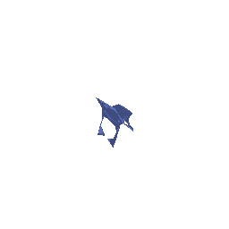
Assumption: how does the amount of visible information in the input view affect the reconstruction of the full 3D shape?

I selected three clearly different views of the same chair and ran the model on each. All predictions are rendered from the same fixed 45° viewpoint so that they can be compared directly. I used the point model.

View 1: Informative perspective view (oblique view where the seat, back and legs are all clearly visible)
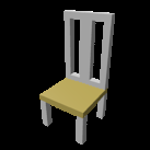
Informative view: input RGB

Input RGB

Informative view: prediction at fixed 45 degree view

Prediction (fixed 45° view)

Informative view: ground truth at fixed 45 degree view

Ground truth (fixed 45° view)

View 2: Front view (some structures overlap)
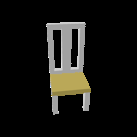
Front/side view: input RGB

Input RGB

Front/side view: prediction at fixed 45 degree view

Prediction (fixed 45° view)

Front/side view: ground truth at fixed 45 degree view

Ground truth (fixed 45° view)

View 3: Blur view (heavy occlusion, only limited geometry visible)
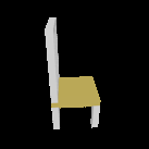
Ambiguous view: input RGB

Input RGB

Blur view: prediction at fixed 45 degree view

Prediction (fixed 45° view)

Ambiguous view: ground truth at fixed 45 degree view

Ground truth (fixed 45° view)

Quantitative results (same chair, F1@0.05):

Input viewF1@0.05
View 1: Informative perspective view98.683
View 2: Front view94.849
View 3: Blur view94.200

Observations:

The F1 score of the point cloud model decreases as the input view shows less of the chair: 98.683 for the informative perspective view, 94.849 for the front view, and 94.200 for the blur view. This is consistent with the idea that a view showing more of the chair gives the model more information to reconstruct the full shape. However, the differences are small, and this test uses a single chair and a single run, so it may not conclusive based on one sample.

3. Exploring other architectures / datasets. (Choose at least one! More than one is extra credit)

3.3 Extended dataset for training (10 points)

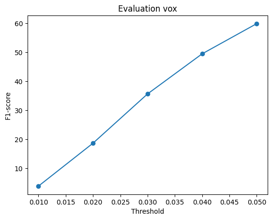
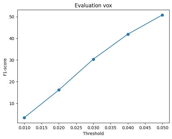
I trained a voxel-based single-view 3D reconstruction model using --load_feat, with the single-class model trained on chairs for 16k iterations and the three-class model trained on chairs, cars, and airplanes for same iterations, and evaluated both models on the same chair test set for comparison.

Quantitative comparison (F1@0.05, same chair test samples):

Training dataF1@0.05
One class (chair)59.840
Three classes (chair, car, plane)50.797

Example 1: model training on class class
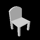
vox example 1: input RGB

Input RGB

vox example 1: Predicted voxel grid

Predicted voxel grid

vox example 1: ground truth mesh

Ground truth

F1@0.05 score: 59.840

F1 plot for single class training model

Example 2: model training on chair car plane classes
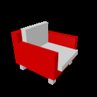
vox example 1: input RGB

Input RGB

vox example 1: Predicted voxel grid

Predicted voxel grid

vox example 1: ground truth mesh

Ground truth

Example 3: model training on chair car plane classes
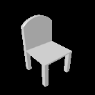
vox example 1: input RGB

Input RGB

vox example 1: Predicted voxel grid

Predicted voxel grid

vox example 1: ground truth mesh

Ground truth

Example 4: model training on chair car plane classes
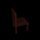
vox example 1: input RGB

Input RGB

vox example 1: Predicted voxel grid

Predicted voxel grid

vox example 1: ground truth mesh

Ground truth

F1@0.05 score: 50.797

F1 plot for three class training model

Analysis:

Training on three classes lowers the F1@0.05 on the same chair test set from 59.840 to 50.797. Both models were trained for the same 16k iterations, so the three-class model knows chairs less, and the generated quality is not as good as the model training on chair class. As the example 1 and 3 show, the model training on chair class has a better result.