A. Neural Volume Rendering
1. Differentiable Volume Rendering
1.3 Ray sampling
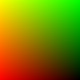
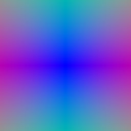
Pixel coordinates are mapped to NDC in [-1, 1], unprojected with the PyTorch3D camera to world-space points on the image plane, and the normalised vector from the camera centre to each point gives the ray direction.
xy_grid |
rays |
|---|---|
 |
 |
1.4 Point sampling
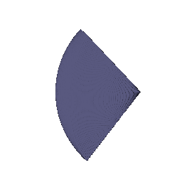
StratifiedRaysampler places n_pts_per_ray evenly spaced depths between near and far and offsets each ray origin along its direction.
1.5 Volume rendering
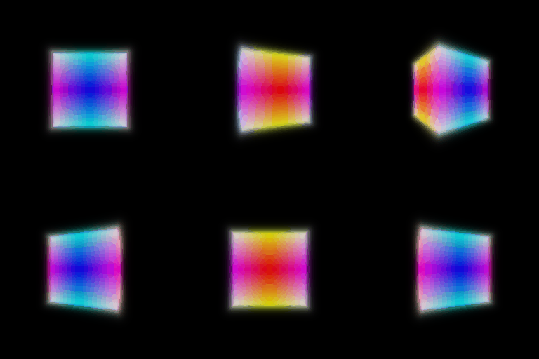
Weights are T · (1 − exp(−σ Δt)), where the transmittance T is the exponential of the (exclusive) cumulative optical thickness along the ray, so the first sample has T = 1. Colour and depth are the weighted sums of per-sample colour and depth; the depth map is normalised by its maximum.
| Spiral rendering | Depth |
|---|---|
 |
 |
2. Optimizing a basic implicit volume
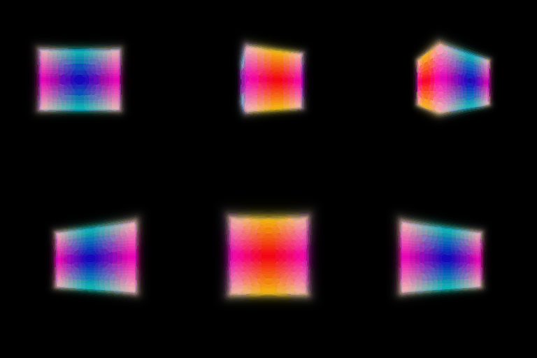
Rays are subsampled with randperm (2.1) and the loss is the MSE between rendered and ground-truth colours (2.2). Training ran for 1,000 epochs with 4,096 rays per step and Adam at LR 5e-4.
Box parameters after training (rounded to 1/100):
- Centre:
(0.25, 0.25, -0.00) - Side lengths:
(2.01, 1.50, 1.50)
| Before training | After training |
|---|---|
  |
  |
3. Optimizing a Neural Radiance Field
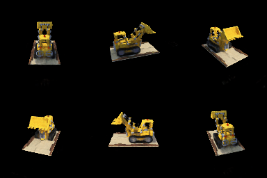
The MLP takes the harmonic embedding of position (6 frequencies, 39-d), passes it through 6 layers of width 128 with the input re-appended at layer 3, and outputs 4 values: ReLU gives density, sigmoid gives RGB. No view dependence. Trained for 250 epochs on 128×128 images with 1,024 rays per step and 128 samples per ray.
4.1 View dependence
Model. View dependence is a switch (implicit_function.use_view_dirs) on the same class, so the position-only model is the exact baseline. When on, the trunk outputs a 128-d feature; density comes from a linear head on that feature (position only), and colour from a small head (one hidden layer of 64) on the feature concatenated with the harmonic embedding of the ray direction (2 frequencies, 15-d). Three choices limit overfitting: density never sees the direction, so geometry is shared by all views; the direction enters late, through a head that can only modulate colour; and the direction encoding has few frequencies, so colour can only vary smoothly with angle.
A practical issue. With this two-linear-layer density path, the pre-ReLU density at initialisation is nearly constant across space and its sign is decided by one random bias. On the mostly-black materials scene a negative start gives an all-black render with zero gradient, which never recovers (the loss sits at ≈0.03 forever). Initialising the density head with small weights and a bias of 0.1 fixes it: training starts as thin uniform fog that the loss carves away.
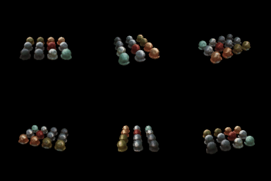
Results on the materials scene (250 epochs each; position-only vs view-dependent, 128 px and 400 px):
| Position only | Position + direction | |
|---|---|---|
| 128×128 | 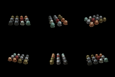 |
 |
| 400×400 | 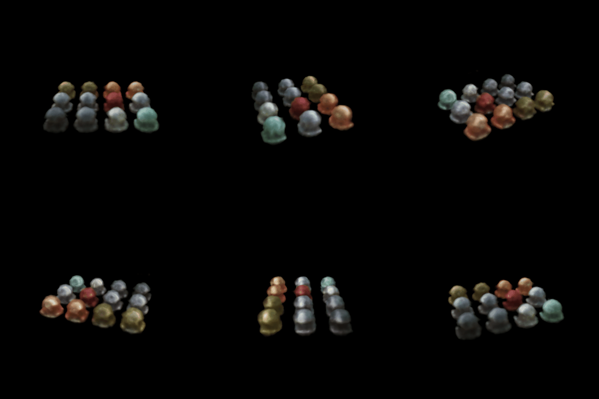 |
 |
Same frames from the 400 px models (left: position only; middle: view-dependent; right: absolute difference), and a zoom of one frame:
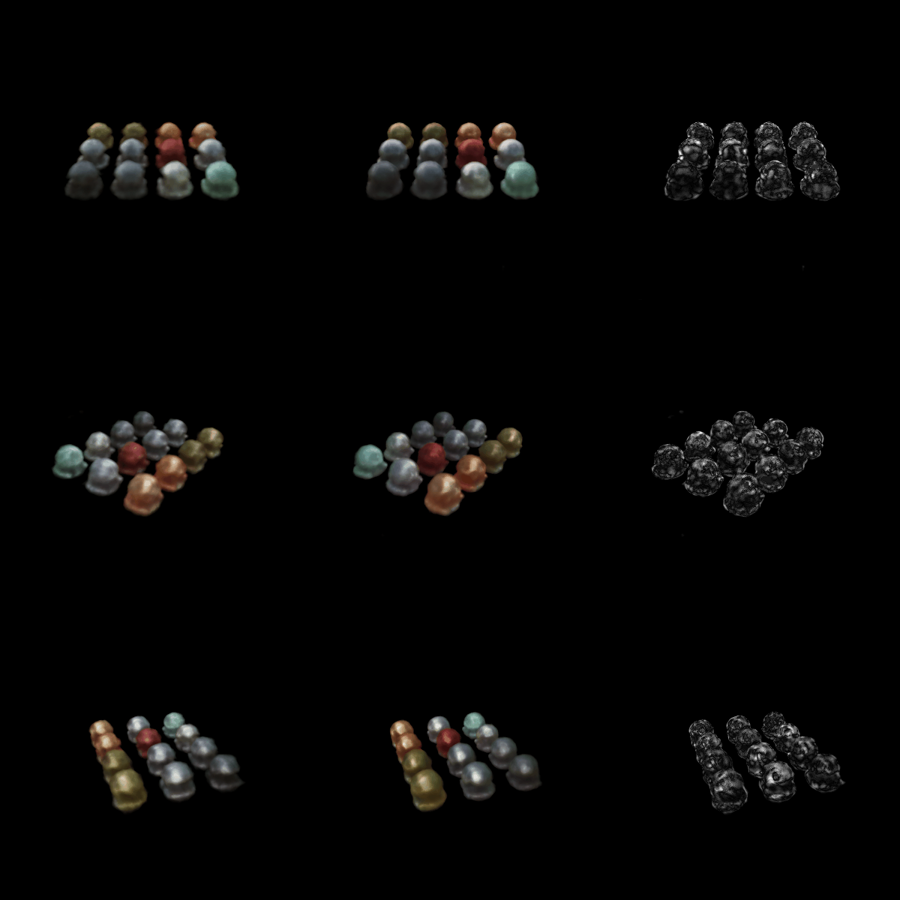
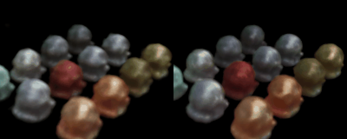
The difference image is zero on the background and brightest at the highlights on the spheres, which is exactly where a view-dependent model should differ. In the zoom, the view-dependent spheres look glossier, with brighter, more localised highlights, while the position-only model paints a dimmer average highlight onto each surface.
Generalisation. PSNR on 10 training views and 20 held-out test views from the dataset's split:
| Model | PSNR train (dB) | PSNR test (dB) | train − test |
|---|---|---|---|
| 128 px, position only | 22.89 | 22.59 | +0.30 |
| 128 px, view-dependent | 24.22 | 23.33 | +0.88 |
| 400 px, position only | 23.51 | 23.04 | +0.47 |
| 400 px, view-dependent | 24.34 | 23.97 | +0.38 |
Trade-offs. View dependence improves held-out views by 0.7–0.9 dB, so with this design it generalises rather than memorises. The cost shows in the train–test gap: at 128 px it grows from 0.30 to 0.88 dB, meaning the model gains more on cameras it has seen than on new ones. That is the trade-off in general: the more freedom colour has to depend on direction (more direction frequencies, a wider head, direction fed earlier), the better the network can fit the exact appearance of each training camera, including effects that are really geometry or noise, and the worse it interpolates between cameras. Keeping the density view-independent and the direction encoding low-frequency buys most of the glossy appearance while keeping that gap small.
B. 3D Gaussian Splatting
5. 3D Gaussian Rasterization
All operations are vectorised over N Gaussians × H·W pixels. The 3D covariance is R diag(s²) Rᵀ (s² I for isotropic Gaussians); the 2D covariance is J W Σ Wᵀ Jᵀ with the provided Jacobian; 2D means come from transform_points_screen; the power is the Mahalanobis form computed with a batched matmul. Gaussians are sorted by view-space depth with z ≤ 0 discarded, alphas are o · exp(power), transmittance is a cumprod over [S, 1−α, …], and image, depth and mask are Σ αᵢTᵢ · {cᵢ, zᵢ, 1}. All 4 unit tests pass.
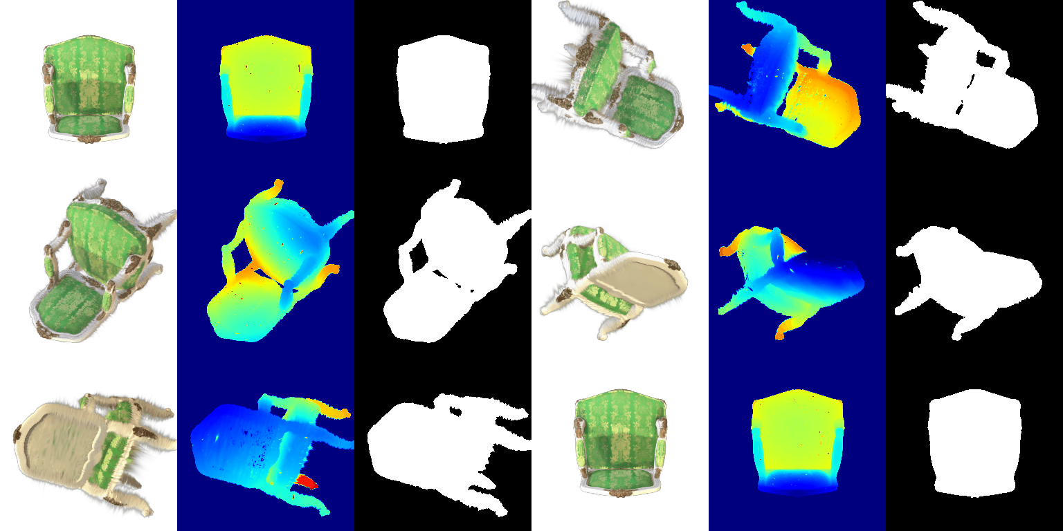
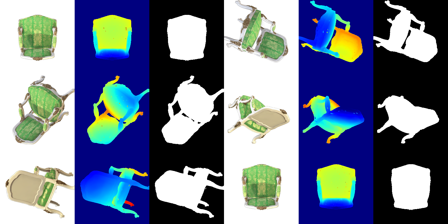
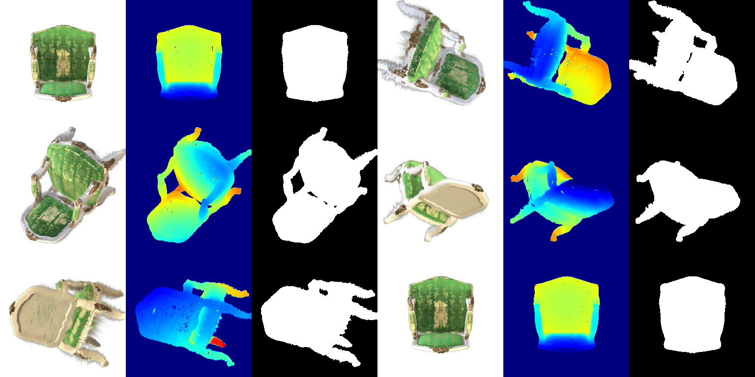
On the rotation convention. Equation (5) of the paper is written for column vectors, where W is the world-to-camera rotation. PyTorch3D stores camera.R for row vectors (X_view = X_world · R + T), so the matrix equation (5) expects is Rᵀ. I checked this two ways: projecting 200k samples from a 3D Gaussian through the camera and measuring their 2D covariance matches J Rᵀ Σ R Jᵀ to within 0.3% and is far from the R version (even the sign of the off-diagonal differs), and renders with Rᵀ are clean while R produces streaks along thin parts (visible on the chair legs and arms above). The provided unit tests 2 and 4, however, were generated with W = camera.R and only pass with it. The submitted code keeps camera.R so the tests pass; the same scene rendered with Rᵀ is shown below for comparison. All later results (sections 6 and 7.1) use camera.R too.
6. Training 3D Gaussian Representations
Setup. Means, scales, colours and opacities are trainable (quaternions are frozen for isotropic Gaussians). Adam with eps=1e-15 and per-parameter learning rates chosen by the units of each parameter:
| Parameter | Learning rate | Reason |
|---|---|---|
| means | 1e-3 | scene units; points are ≈0.03 apart, so a step should stay well below that |
| scales (log) | 5e-3 | ≈0.5% size change per step |
| colours | 2e-2 | RGB in [0, 1], initialised at random, must travel ≈0.5 |
| opacities (logit) | 5e-2 | initialised at 8.0, deep in the sigmoid's flat tail |
L1 loss on RGB with a black background, 1,000 iterations, all Gaussians splatted per call.
Held-out metrics (mean over the test views): PSNR = 29.83 dB, SSIM = 0.941.
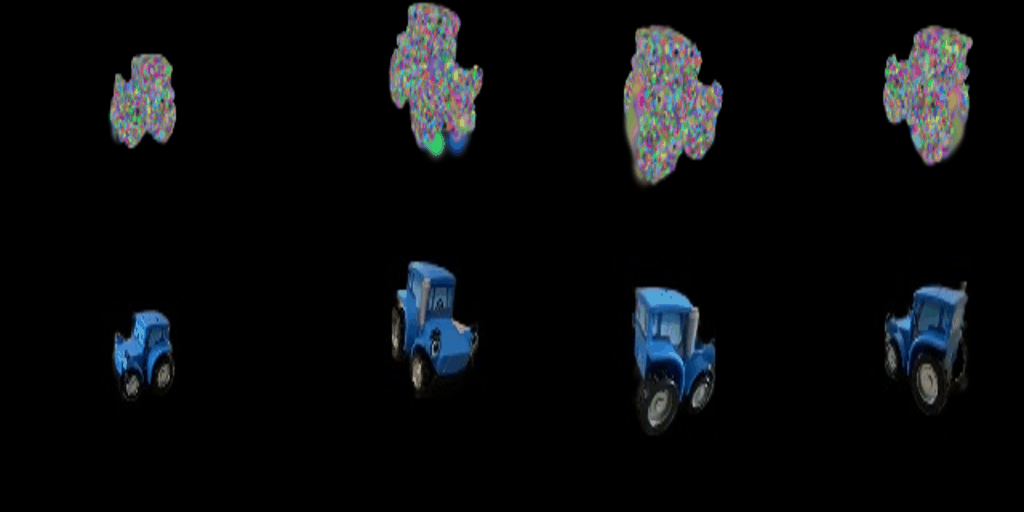
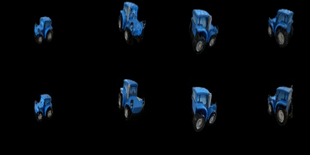
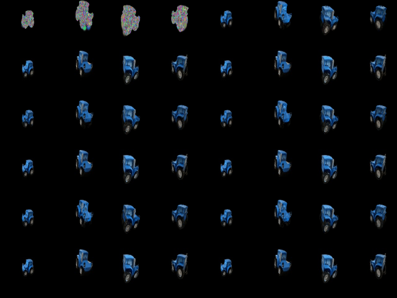
Training progress (top: renders during training; bottom: ground truth), first and last frame, and the full GIF:
Final renders of the training views:

7.1 Rendering using spherical harmonics
Each Gaussian carries 16 degree-3 SH coefficients per colour channel (48 values). Colour is evaluated per Gaussian along the normalised world-space direction from the camera centre to the Gaussian, using the standard real-SH constants and ordering, with the same +0.5 offset and clamp as the DC colour. With all higher-order coefficients zeroed this reduces exactly to the section 5 colours, which served as the check.
| DC only (section 5) | Full SH (7.1) |
|---|---|
|
 |
Side-by-side frames at the same indices (left: DC only; right: full SH). Both are rendered with the same camera.R convention, so the only change is the colour model.

Frame 1. The damask pattern on the back and seat gains contrast: the gold motifs are brighter and the green between them deeper. The DC colour is an average over all directions, which washes the pattern out; from this near-frontal view the SH terms recover the sheen of the fabric.
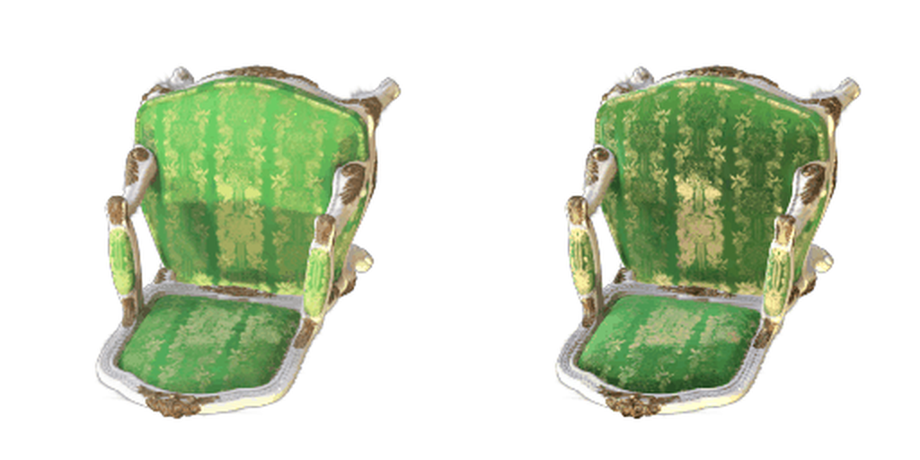
Frame 14. A view from above and behind. The seat cushion shows a broad bright patch under SH that is absent in the DC render: a view-dependent sheen on the silk that only appears at grazing angles. The gilded carving on the arms also looks warmer and more saturated.
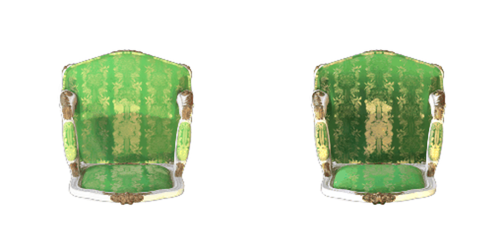
Frame 31. Near-frontal again. The SH render has a bright highlight in the centre of the back cushion and darker edges, consistent with fabric lit from the front; the DC render is uniformly flat. The white frame is almost identical in both, as expected for a matte surface whose SH coefficients are dominated by the DC term.
Overall, SH mostly changes the shiny parts (silk and gilding) and leaves matte parts alone, and the differences move with the camera, which is what a view-dependent colour model should do.