1. Differentiable Volume Rendering
1.3 Ray sampling
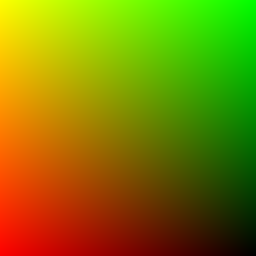
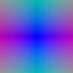
I implement get_pixels_from_image to map pixel coordinates to NDC, and get_rays_from_pixels to unproject them with camera.unproject_points into rays from the camera centre. Both visualizations match the TA images.
1.4 Point sampling
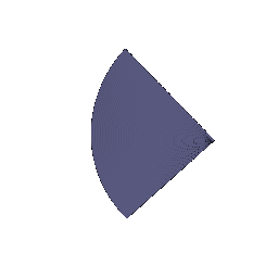
I implement StratifiedRaysampler to place n_pts_per_ray depths uniformly between min_depth and max_depth and sample points at origin + depth × direction.
1.5 Volume rendering
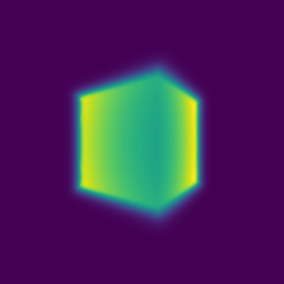
I implement _compute_weights and _aggregate as the weighted sum along each ray. The same weights render the color and the depth.

2. Optimizing a Basic Implicit Volume
2.1 Random ray sampling
I implement get_random_pixels_from_image to pick n_pixels random pixels from the full grid, so each step renders only a batch of rays.
2.2 Loss and training
I define the loss as the MSE between the rendered colors and rgb_gt. After training, the box is:
Box center: (0.25, 0.25, 0.00)
Box side lengths: (2.01, 1.50, 1.50)
2.3 Visualization
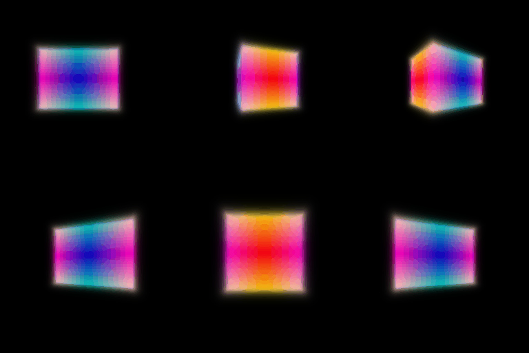
The spiral rendering of the optimized box matches the TA GIF in shape, size and position.
3. Optimizing a Neural Radiance Field (NeRF)
Network. Positional encoding of xyz (6 frequencies) → 6-layer MLP (128 units, skip connection at layer 3) → ReLU density head and sigmoid color head. Loss. MSE on 1024 random rays per step.
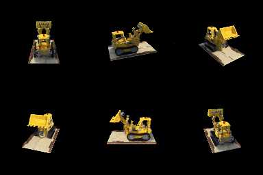
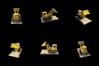
nerf_lego.yaml, 128x128, 250 epochs).The rendering matches the TA reference: the shape of the bulldozer, the yellow body, the dark treads and the textured base are all reconstructed, and the test PSNR is 24.50 dB.
4. NeRF Extras
4.1 View Dependence
Network. Following the NeRF paper, I feed the encoded viewing direction only into the color head, after the density head. The density depends only on the position, so the network cannot overfit the training views with view-dependent geometry.
L is the number of frequencies in the harmonic encoding of the viewing direction d: γ(d) = (d, sin(2^0 d), cos(2^0 d), …, sin(2^(L−1) d), cos(2^(L−1) d)), which has 3 + 6L dimensions. A larger L lets the color change faster as the viewpoint moves, so it can represent sharper highlights but can also fit view-specific details of the training images. The baseline without view dependence ignores the direction entirely.
I trained on the materials scene (nerf_materials.yaml, 128x128, 1000 epochs, learning rate 5e-4) without view dependence and with L = 2, 4 and 8. The highlight PSNR is computed only on the brightest pixels (any channel above 0.8), which are the specular highlights.
| Model | Train PSNR | Test PSNR | Train-test gap | Highlight PSNR (train / test) |
|---|---|---|---|---|
| No view dependence | 25.88 | 24.26 | 1.61 | 11.60 / 11.63 |
| L=2 | 28.51 | 26.27 | 2.24 | 15.37 / 13.94 |
| L=4 | 28.69 | 26.31 | 2.38 | 16.04 / 14.10 |
| L=8 | 28.88 | 26.23 | 2.65 | 15.97 / 13.98 |


Trade-off between view dependence and generalization:
- View dependence improves the test views. Adding it raises test PSNR by about 2 dB and highlight PSNR by 2.3–2.5 dB. Without it, the specular highlights are averaged into a dull, view-independent color (Figure 6).
- More view dependence widens the train-test gap. Train PSNR keeps rising with L, but test PSNR stops improving after L=2, so the gap grows at every step. The extra directional detail fits the training views without generalizing to new viewpoints. The highlights show this clearly: with view dependence, they are about 1.5–2 dB worse on the test views than on the training views, while without it they are equally poor on both.
- The network uses mostly the low frequencies. In the L=8 model, the color-layer weights on the three lowest frequencies (2^0–2^2) grew to about 5 times their initial size and those on 2^3 to about 3 times, while those on 2^6 and 2^7 stayed at their initial size.
In summary, a small L (2–4) gives most of the benefit, and a larger L mainly widens the train-test gap. Even so, the mirror-like reflections stay blurrier than the ground truth (Figure 6). The reflected image changes very sharply with both the viewing direction and the position, which this small color head cannot represent.
4.2 Coarse/Fine Sampling
Sampling. A coarse network is evaluated at 64 stratified samples. I draw 128 more samples from its rendering weights by inverse-transform sampling (sample_pdf), and a fine network is evaluated at all 192. Loss. MSE on both renderings. The figure compares uniform 128 samples (Q3), uniform 192, and coarse 64 + fine 128.
| Sampling Scheme | Test PSNR | Train Step (ms) | Render 128px (s) | # Params |
|---|---|---|---|---|
| uniform_128 (Q3) | 24.497 | 8.1 | 0.031 | 117,764 |
| uniform_192 | 24.754 | 12.95 | 0.049 | 117,764 |
| coarse_64 + fine_128 | 24.936 | 16.26 | 0.061 | 235,528 |

- Quality: coarse/fine improves test PSNR by 0.44 dB over uniform 128, and by 0.18 dB over uniform 192, which uses the same total number of samples. The gain comes from placing samples near the surface instead of in empty space.
- Speed: each step runs two networks and an extra sampling pass, so training takes 2.0× as long per step as uniform 128 (1.3× as long as uniform 192). Rendering is slower by a similar factor, and the model has twice as many parameters.
Coarse/fine sampling is worth the cost when quality matters. When speed matters, adding uniform samples recovers part of the gain more cheaply.
4.3 VolSDF
I implement VolSDF following items described in the instructions:
- Network. Positional encoding → distance MLP (6 layers, 128 units, linear output) and color MLP (2 layers, sigmoid output).
- Eikonal loss. mean((‖∇d‖ − 1)²) on random points.
- SDF to density. σ(x) = α Ψ_β(−d(x)), where Ψ_β is the Laplace CDF with scale β.
- α is the density inside the object (σ = α deep inside, α/2 on the surface).
- β is the width of the transition from empty to solid. As β approaches to 0, the surface becomes perfectly sharp.
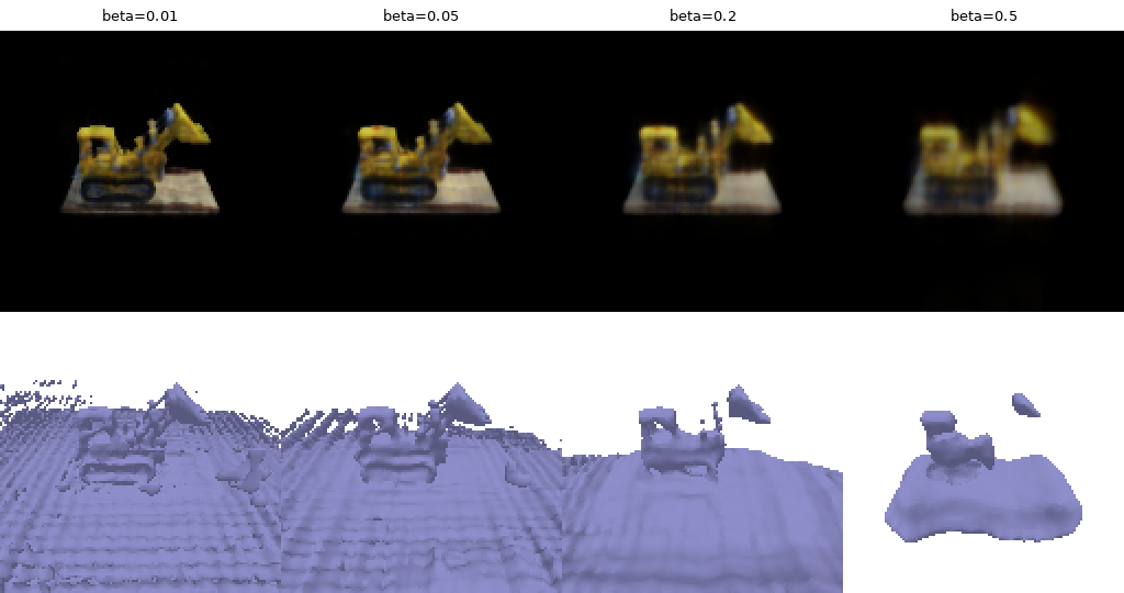
I sweep β from 0.01 to 0.5 (α = 10). Depth gap is the distance between the rendered depth and the SDF zero crossing. Empty-ray opacity is the opacity of rays that miss the surface (haze).
| β | Test PSNR | Depth gap | Empty-ray opacity |
|---|---|---|---|
| 0.01 | 21.21 | 0.099 | 0.003 |
| 0.05 | 20.96 | 0.089 | 0.043 |
| 0.2 | 20.13 | 0.216 | 0.465 |
| 0.5 | 18.70 | 0.395 | 0.679 |

- How does β bias the SDF? High β spreads density away from the zero level set, so the SDF learns a bloated shape that loses thin parts (Figure 9, β ≥ 0.2). Low β makes the rendered surface coincide with the zero level set, so there is little bias.
- Which is easier to train? High β. Many samples along each ray get gradients, even when the surface is far from where it should be. With low β, only samples within ~β of the surface get gradients, and β = 0.01 is smaller than the sample spacing (0.03).
- Which gives a more accurate surface? Low β. Rendering is determined by the zero level set itself, so fitting the images places it on the true surface. This gives the sharpest mesh and no haze.
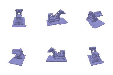
Settings. α = 10, β = 0.01, eikonal weight 0.02, 250 epochs. The key change is a geometric initialization (from IDR/VolSDF) that starts the network as the SDF of a sphere. With random initialization, unconstrained regions keep random zero crossings, which become spurious surfaces in the mesh (Figure 10). I kept the default α = 10: a ray is about 95% opaque within 0.3 units (about 10 samples) past the surface, so the color comes from a thin shell at the surface. I also kept the default eikonal weight of 0.02, which keeps ‖∇d‖ close to 1 so that d stays a true distance and β keeps its meaning, without overpowering the color loss.
5. 3D Gaussian Rasterization
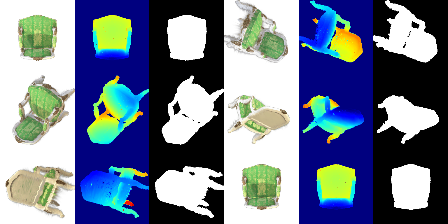
I implement the rasterizer in model.py and render.py, vectorized over all Gaussians:
- Projection. Each 3D Gaussian is projected to a 2D Gaussian on the image plane.
- 2D evaluation. Each 2D Gaussian is evaluated at every pixel. All 4 unit tests pass.
- Sorting. Gaussians are sorted by depth, and those behind the camera are dropped.
- Splatting. Front to back, each Gaussian's opacity and the remaining transmittance weight its color, depth and mask.
The GIF shows the color, depth and mask of the pre-trained chair rendered by render.py.
6. Training 3D Gaussian Representations
I train 10,000 isotropic Gaussians on the toy truck, initialized from the provided point cloud.
6.1 Parameters and optimizer. make_trainable makes the means, scales, opacities and colors trainable, and setup_optimizer uses Adam with a learning rate per parameter:
| Parameter | Learning rate |
|---|---|
| Opacities | 0.005 |
| Scales | 0.01 |
| Colors | 0.005 |
| Means | 0.01 |
The starter rate of 0.05 was too high, so I lowered all of them, most for the colors and opacities.
6.2 Forward pass and loss. Each iteration renders one training view with scene.render and computes the MSE against the ground truth.
| Iterations | PSNR | SSIM |
|---|---|---|
| 1000 | 28.903 | 0.926 |
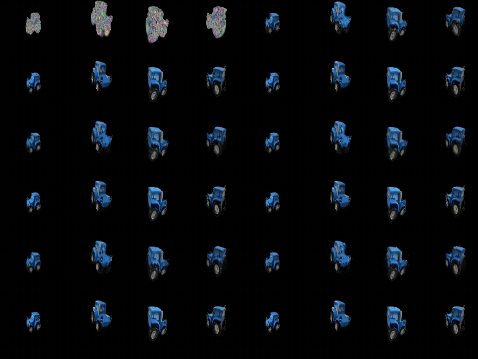
At iteration 0 the Gaussians already form the truck, since they start from the point cloud, but their colors are random. The colors and silhouette match the ground truth after about 200-300 iterations, and the rest of training sharpens details such as the wheels and windows.

7. Extensions
7.1 Rendering Using Spherical Harmonics
I implement colors_from_spherical_harmonics, which evaluates spherical harmonics up to degree 3 along the direction from the camera to each Gaussian. The baseline (Q5.5) uses only the degree-0 term, which is the same from every direction.

Side-by-side comparison of the same frames, with the baseline (top) and with spherical harmonics (bottom):

- Frame 012: The reflections are much clearer with spherical harmonics. The gold decorations on the armrests and along the edges of the seat frame show bright, sharp highlights next to darker areas. In the baseline, the gold looks flat and evenly lit. Reflections depend on the viewing direction, so the baseline cannot show them, because each Gaussian has the same color from every direction.
- Frames 015 and 017: These two frames show the same seat from different directions. In the baseline, the seat looks about equally bright in both frames. With spherical harmonics, the seat is clearly darker in frame 015 than in frame 017. That is because the brightness changes with the viewing direction, which only spherical harmonics can represent.
7.2 Training On a Harder Scene
Both methods start from 10,000 random Gaussians and train for 5000 iterations. The table below shows the parameters used for each training configuration.
| Baseline (Q6 setup) | Improved | |
|---|---|---|
| Learning rates | opacities 0.005, scales 0.01, colors 0.005, means 0.01 | opacities 0.05, scales 0.005, colors 0.01, means 0.005 → 0.00005, quaternions 0.001 |
| Iterations | 5000 | 5000 |
| PSNR | 21.430 | 24.381 |
| SSIM | 0.626 | 0.891 |
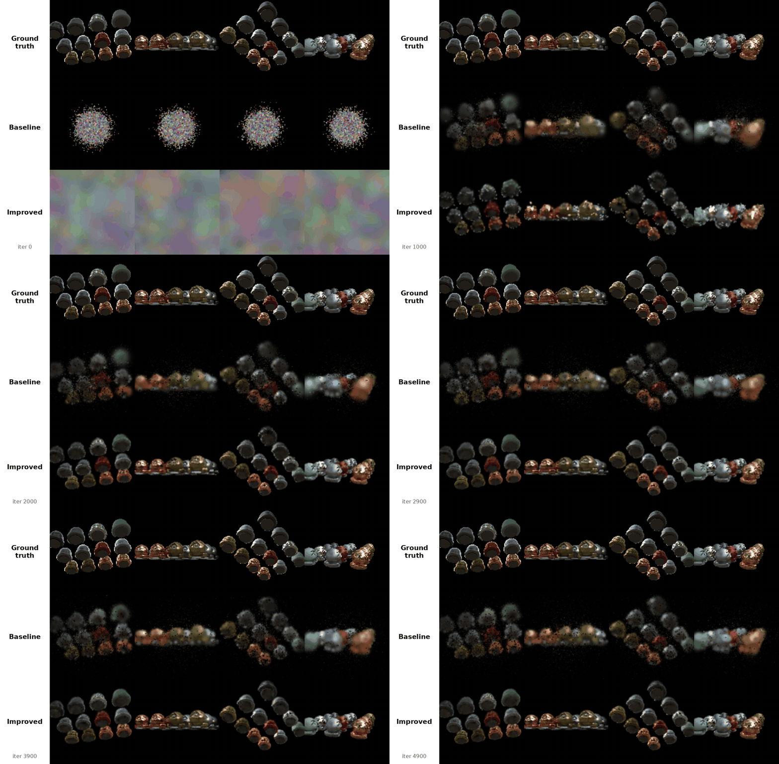


The baseline Gaussians start as a small ball and stay speckled and noisy. The improved Gaussians cover the scene from the start, place the objects within about 500 iterations, and end much sharper.
Modifications compared with Q6:
- Initialization: means uniform over the whole scene (a cube of half size 1.5) instead of a small ball, scales from the distance to the nearest neighbors, and a low initial opacity (0.1).
- Anisotropic Gaussians: a scale per axis plus a rotation, to fit edges and surfaces.
- L1 + D-SSIM loss (weight 0.2 on D-SSIM), as in the original paper.
- Learning-rate schedule: the means' learning rate decays exponentially by 100× over training.
- Simplified adaptive density control: every 200 iterations from 500 to 3000, the 5% of Gaussians with the largest mean gradient are cloned (if small) or split (if large). Nearly transparent or very large Gaussians are pruned.