
vis_grid)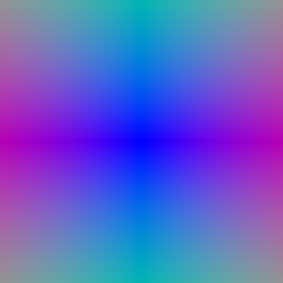
vis_rays)vis_grid)vis_rays)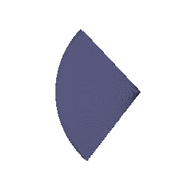

part_1.gif)
After training the box volume for the provided number of iterations:
| x | y | z | |
|---|---|---|---|
| Box center | 0.25 | 0.25 | −0.00 |
| Box side lengths | 2.01 | 1.50 | 1.50 |

part_2.gif)The TA's Gif and my Gif look almost identical to me, with everyhting like size colour shape matching. The only difference might be in position but that also looks very similar.
Training views before and after optimisation (top: before, bottom: after):


The NeRF is an MLP on harmonic-embedded positions (6 frequencies; 39 input features, including the raw xyz). A density head (a linear layer from the 128-d feature to 1 output, bias initialised to 1.0, followed by ReLU so density is non-negative) and a colour head (a 128→64 linear layer, ReLU, a 64→3 linear layer, and a sigmoid so RGB is in [0, 1]) both read this feature. The loss is the mean squared error between rendered and ground-truth pixel colours over 1024 random rays per step, optimised with Adam (lr 5e-4, decayed by 0.8 every 50 epochs) for 250 epochs on 128×128 lego images with 128 samples per ray.

Design. Following the original NeRF, density depends only on position and is computed before the viewing direction is used. The (harmonic-embedded, 2 frequencies) view direction is concatenated to the position feature only in a shallow colour head (64 hidden units).
Setup. nerf_materials config: 128×128 images, 250 epochs, 128 samples per ray, black background (white_background: False), lr 5e-4. Though I tried with the white backgroud but the results were poor.

Trade-offs. View dependence lets the colour of a surface change with the viewing direction, which is what makes glossy and metallic materials look right, and it highlights areas on the surface as the camera moves. Without it, the network has to explain every training view with jsut one colour per 3D point, so glossy regions come out as flat wtih matte look. The downside of it is the capacity that can be spent on memorising training views: a view-dependent colour function can reproduce each training image without a consistent geometry, which hurts novel views.
One of the mistakes I did, My first materials runs trained against a target I had composited onto a white background while the renderer returned black for empty space (white_background: False). The network could only match the target by filling empty space with bright fog, so the outputs were washed out (white fog in most frames). I then fixed this using the starter's loader (black background) with white_background: False. The test GIF is rendered from the hard-coded spiral cameras of train_nerf; I matched its focal length to the dataset's cameras (3.125) for the materials scene so the objects fill the frame as in the training images.
A coarse network renders 64 uniformly stratified samples per ray. Its weights define a piecewise-constant PDF along the ray, from which 64 additional depths are drawn by inverse-CDF sampling. The coarse and fine depths are merged and sorted and passed to a separate fine network. The loss is the sum of the coarse and fine MSE. Total samples per ray stay at 128, so the baseline is 128 uniform samples with one network.

| Baseline (128 uniform) | Coarse/fine (64 + 64) | |
|---|---|---|
| Validation PSNR (100 views, epoch-200 checkpoint) | 24.30 dB | 24.69 dB |
| Render time per image (128×128) | 0.16 s | 0.31 s |
| Parameters | 96,260 | 192,520 |
| Training time (250 epochs) | 18 min 19 s | 24 min 07 s |
Trade-offs. Coarse/fine concentrates the second set of samples where the coarse pass found density, so the same sample budget is used where it matters. It improved validation PSNR by 0.39 dB. The price is a second network (twice the parameters), a second sequential pass with a sort, about 1.9×, the render time per image and about 1.3× the training time. The gain is modest here: the scene is rendered at low resolution with a small MLP. I did not test this, but I would expect coarse/fine sampling to help more when the occupied part of each ray is small compared with the sampled depth range (large empty regions) or at higher resolution, where finer detail is visible and uniformly spaced samples are more likely to step over thin surfaces. The coarse pass finds where the density is along each ray, and the fine pass places its samples there instead of spreading them uniformly over empty space.
Implementation. The surface is a signed-distance MLP: harmonic embedding of xyz (6 frequencies), six 128-unit layers with Softplus activations (smooth, so the eikonal term has useful second derivatives), a linear output so the distance can be negative, and a colour head that shares the trunk features. The distance is converted to density with the Laplace CDF used in VolSDF:
density = α · (0.5 · exp(−d/β) if d > 0 else 1 − 0.5 · exp(d/β)).The eikonal loss mean((||∇f|| − 1)²), weight 0.02, is applied at random points in the box [−4, 4]³.
Best result (α = 10, β = 0.05).


Final per-epoch training loss: roughly 0.005 - 0.008 for β = 0.05 and 0.03 - 0.06 for β = 0.5 (single-batch values, so noisy).
What α and β do. The density is α times the CDF of a Laplace distribution (scale β) evaluated at the negative signed distance. α is the density deep inside the object, so it controls how opaque the interior is (a large α means rays are absorbed immediately once they enter). β controls how sharply density changes at the surface: the density is exactly α/2 on the zero level set, and it reaches roughly α and 0 at a distance of a few β inside and outside.
1. How does a high β bias the learned SDF? What about a low β? A high β makes the density change slowly with distance, so the rendered image is a blurred version of the object, and the SDF is pushed toward an over-smooth, "inflated" surface: fine details are lost and thin parts are rounded off. A low β ties the rendering tightly to the exact location of the zero level set, so the SDF can represent sharp detail, but it is biased toward noisy or fragmented surfaces when the data does not constrain it: it only receives a signal from samples that land within a thin band.
2. Is an SDF easier to train with volume rendering at a low or a high β? In principle a high β is easier to optimise: the density changes slowly with distance, so many samples along each ray carry non-trivial density and gradients reach points far from the surface. My experiments did not show this. With β = 0.5 the training loss stayed at 0.03–0.06 and the output was not recognisable, while β = 0.05 reached 0.005–0.008 and gave a clean result. I believe this is because a band as wide as β = 0.5 is a large fraction of the object’s size, so the density cannot represent a sharp object boundary and the images cannot be matched closely. A much smaller β (0.01) failed in a different way: the loss became NaN within a few epochs, caused by exp(d/β) overflowing in the unused branch of torch.where (the backward pass multiplies zero by infinity).
3. Which β is more likely to learn an accurate surface? Why? A low β, as long as training is stable, with density concentrated at the zero level set, the render depends on the exact position of the surface, so the surface can be sharp and accurate. A high β cannot localise the surface better than the width of its band. In practice there is a trade-off, and a moderately small β usually works best.
Settings I chose, and why. I kept α = 10 and chose β = 0.05 after comparing it with β = 0.5. With β = 0.05 the final training loss was about 0.005 - 0.008, compared with 0.03 - 0.06 for β = 0.5, and the geometry is visibly sharper. A much smaller β (0.01) did not work for me: training produced NaN losses within a few epochs and an unrecognisable output. The other settings are the starter's defaults: eikonal weight 0.02, lr 5e-4 with 0.8 decay every 50 epochs, 250 epochs, 128 samples per ray, a 6-layer, 128-unit SDF MLP. I tried experimenting with it a bit, including changing LR and decay but the starter's default one worked best for me.

| Parameter | Learning rate |
|---|---|
| Opacities | 0.05 |
| Scales | 0.01 |
| Colours | 0.02 |
| Means | 0.001 |
Adam with a per-parameter learning rate and an exponential decay to 5% of the initial rate over training (ExponentialLR, γ = 0.051/N), isotropic Gaussians, L1 loss, 1000 iterations, splatting in mini-batches of 1000 Gaussians. PSNR 29.068, SSIM 0.937.
My first attempt used 0.05 for every parameter and plateaued at a loss of about 0.015; a smaller learning rate for means and scales plus the decay fixed this.


Side-by-side frames (left: without SH, right: with SH):


As we can see, in all three frames, the renderings with spherical harmonics (SH) show a clearly visible colour shift compared with the DC-only renderings, and the brighter regions fade into the shadowed regions much more naturally, instead of looking like flat patches of constant colour. Mainly the difference is visible in shading of the regions.
Settings for all runs: 128×128 images, 10,000 isotropic Gaussians with init_type="random", Q6 learning rates, and the L1 loss, splatting in mini-batches of 500 Gaussians (limited by an 8 GB GPU). All runs (baseline and improved) were trained for 1000 iterations. The improved run used the same learning rates as the baseline and Q6: opacities 0.05, scales 0.01, colours 0.02 and means 0.001, with the same exponential decay to 5% of the starting rate. The improved run changes only the initialisation (below); the baseline and the improved run are evaluated on held-out views of the materials scene.
| Run | PSNR | SSIM |
|---|---|---|
| Baseline (Q6 setup, default random init) | 18.024 | 0.654 |
| Attempt A: dense, opaque random init | 17.436 | 0.456 |
| Improved (attempt B) | 22.251 | 0.800 |
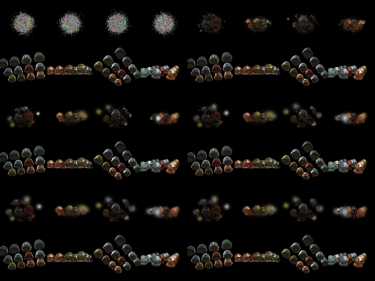
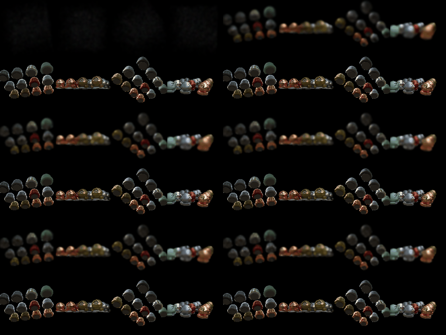


Comparison. The improved run raises PSNR from 18.02 to 22.25 dB and SSIM from 0.654 to 0.800. The improved run trains very differently from the baseline: clear blob-like shapes appear very early in the progress GIF, whereas the baseline stays blurry. The blobs in the improved run are also sharper and better rounded, while the baseline renders them as soft, smeared patches.
What I changed for the improved run. Inspecting the scene showed the camera is about 4 units from the origin, and that 75% of pixels are black (mean pixel value 0.07). With random initialisation, the baseline's Gaussians were dense, opaque and bright, so along each ray the first layer absorbed nearly all transmittance and only the front Gaussians received gradient. My modifications to the initialisation:
Attempt A (dense and opaque, in the same spread) made things worse (PSNR 17.4, SSIM 0.456), which confirmed the transmittance-collapse explanation: the opacity and scale initialisation mattered, not just the spread.