
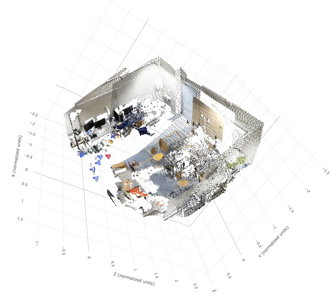


The following visualizations were generated after the unprojection stage (left) and canonicalization stage (right) for each scene. The first camera center is shown in red, and the other camera centers are shown in blue, in each image.
| Unprojection Image | Canonicalization Image |
|---|---|
|
|
|
|
|
|
|
|
|
|
The following output was generated from the
check_data.py script.
{
    "sequence_name": "e050c15a8d_frame_007080",
    "views": 8,
    "resolution": 224,
    "valid_depth_fraction": 0.9779127240180969,
    "max_reprojection_error_px": 0.00011009880108758807,
    "max_ray_reprojection_error_px": 9.448717901250347e-05,
    "centroid_distance": 1.0
},
{
    "sequence_name": "5f99900f09_frame_002820",
    "views": 8,
    "resolution": 224,
    "valid_depth_fraction": 0.9903116226196289,
    "max_reprojection_error_px": 0.00011108566104667261,
    "max_ray_reprojection_error_px": 0.00011108566104667261,
    "centroid_distance": 0.9999999403953552
},
{
    "sequence_name": "47b37eb6f9_frame_002720",
    "views": 8,
    "resolution": 224,
    "valid_depth_fraction": 0.9609947800636292,
    "max_reprojection_error_px": 9.591897105565295e-05,
    "max_ray_reprojection_error_px": 8.897326188161969e-05,
    "centroid_distance": 1.0
},
{
    "sequence_name": "4c5c60fa76_frame_006690",
    "views": 8,
    "resolution": 224,
    "valid_depth_fraction": 0.7516716122627258,
    "max_reprojection_error_px": 0.0001089862416847609,
    "max_ray_reprojection_error_px": 0.00010141761595150456,
    "centroid_distance": 0.9999999403953552
}
In this output you can see that the centroid distance rounds to 1.0 for each image, and the max reprojection error and max ray reprojection errors are near-zero, meaning the implementation is working as intended.
As an explanation of the terms above, canonicalization represents all poses relative to camera 0 by adjusting the rotation, scale (depth), and translation data. World-space ray directions are a way to project each pixel inversely through the camera intrinsics, rotating and normalizing by the camera only, and keeping the camera center as the origin. Plucker moment refers to the cross product of the world-space ray origins and the world-space ray directions, which returns a point in space independently of which point along the ray you consider to be origin.
Implemented task 2.0 and ran the overfitting script, resulting in the following values.
Final overfit training loss: 0.00574.
Final overfit training PSNR: 27.32.
Final overfit validation loss: 0.00041.
Final overfit validation PSNR: 33.95.
The val_epoch000.png that was produced is shown below.

The training curves below show the training and validation loss / PSNR with over time, and demonstrate that loss decreased and PSNR increased over time, as expected.


The following table is the resulting evaluation with different number of source views and different ablations. Each target-ray conditioning type is shown in the columns, and each number of source views is shown in the rows.
PSNR Table
| None | Shuffled | Correct | |
|---|---|---|---|
| 1 source views | 12.47 | 11.82 | 15.13 |
| 2 source views | 12.43 | 11.50 | 16.03 |
| 4 source views | 12.48 | 11.67 | 16.76 |
SSIM Table
| None | Shuffled | Correct | |
|---|---|---|---|
| 1 source views | 0.53 | 0.49 | 0.56 |
| 2 source views | 0.53 | 0.48 | 0.56 |
| 4 source views | 0.54 | 0.48 | 0.58 |
Below is the training validation output prdouced at epoch 100.

Below are the eval validations produced for varying numbers of source views and target-ray conditioning types.
1 source view, none conditioning type

1 source view, shuffled conditioning type

1 source view, correct conditioning type

2 source view, none conditioning type

2 source view, shuffled conditioning type

2 source view, correct conditioning type
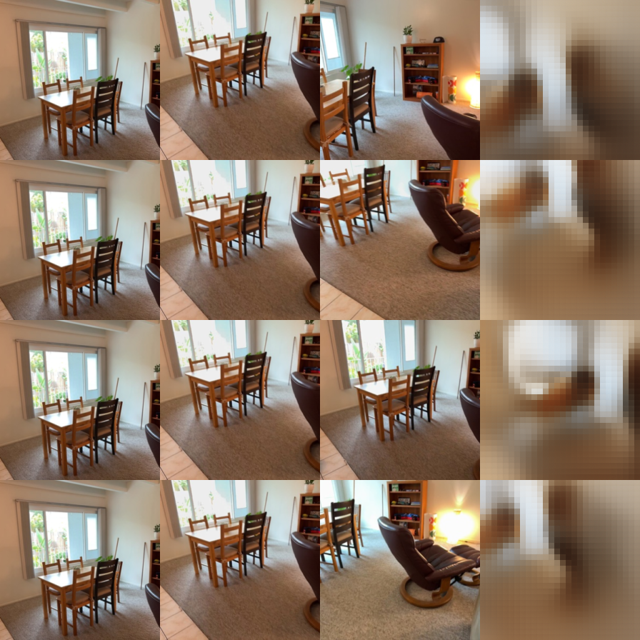
4 source view, none conditioning type

4 source view, shuffled conditioning type

4 source view, correct conditioning type

The config I used was the default config (100 epochs, 0.0002 lr, etc.), except to get it to train on my laptop, I had to reduce the batch size from 4 to 2 so that it would fit within my GPU’s memory limit.
Looking at the PSNR and SSIM table, we can see that the using the true target rays (correct) performed best, followed by using all-zero rays (none), and finally rays of a different target (shuffled). Also, the results show that the number of source views didn’t have any effect on the PSNR or SSIM of the output, likely because the network was only trained on a constant number of source views (2). Visually, however, the output does seem to improve when more source views are provided.
I investigated the training view count direction. Specifically, I
asked the question, what would happen if a variable number of training
views were provided during the training process itself? I implemented
the code configuration such that an array of source views could be taken
in at runtime, and each iteration a random number from that array would
be chosen to determine how many source views to provide. I used
[1, 2, 4]. All other config parameters were the same as
section 2.2.
Below are the validation loss and PSNR curves over the training epochs.


The metrics were close, but slightly better than the baseline (section 2.2). Below is the SSIM and PSNR ablation table for the correct target-ray conditioning type.
| SSIM | PSNR | |
|---|---|---|
| 1 source views | 0.56 | 15.15 |
| 2 source views | 0.57 | 16.02 |
| 4 source views | 0.59 | 16.69 |
The numbers improve slightly, indicating that performance improved, but not significantly. In the shuffled and none conditioning type, there was no difference whatsoever. The images below show the new predictions for the correct conditioning type.
1 source view

2 source view
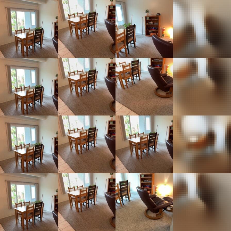
4 source view

This lack of significant difference is visualized here, as the images are very similar to those generated by baseline. I was hoping for a more significant improvement in the 1 and 4 source view cases, since those were now part of the training data, but there wasn’t much improvement in those scenarios. However, this does make sense since even in the baseline scenario, the different number of source views didn’t significantly affect the PSNR, SSIM, or visualization in any way.
After the 40 epochs of overfit training, the final training loss was -0.173, with a final camera loss of 0.003 and a final depth loss of -0.186. The image below shows the training curves for overall loss, camera loss, and depth loss.

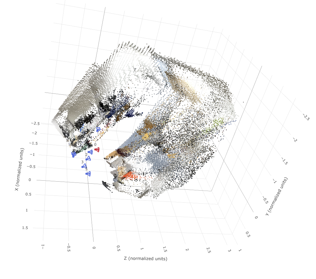
Below are screenshots showing the ground-truth 3D image (top), as well as the predicted camera + depth image (bottom).

The training and validation loss curves after 250 epochs of training are shown below for overall loss, camera loss, and depth loss.

The tables below show the specified metrics, on both the validation and test sets.
Metrics Table
| Validation | Test | |
|---|---|---|
| Depth AbsRel | 0.168 | 0.183 |
| Depth δ1 | 0.00 | 0.773 |
| Rotation AUC 5° | 0.122 | 0.122 |
| Rotation AUC 15° | 0.372 | 0.371 |
| Rotation AUC 30° | 0.559 | 0.605 |
| Translation AUC 5° | 0.006 | 0.003 |
| Translation AUC 15° | 0.041 | 0.037 |
| Translation AUC 30° | 0.121 | 0.115 |
| Joint Pose AUC 5° | 0.002 | 0.001 |
| Joint Pose AUC 15° | 0.031 | 0.023 |
| Joint Pose AUC 30° | 0.104 | 0.097 |
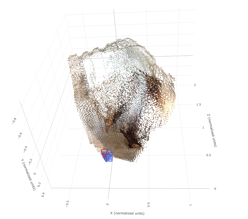
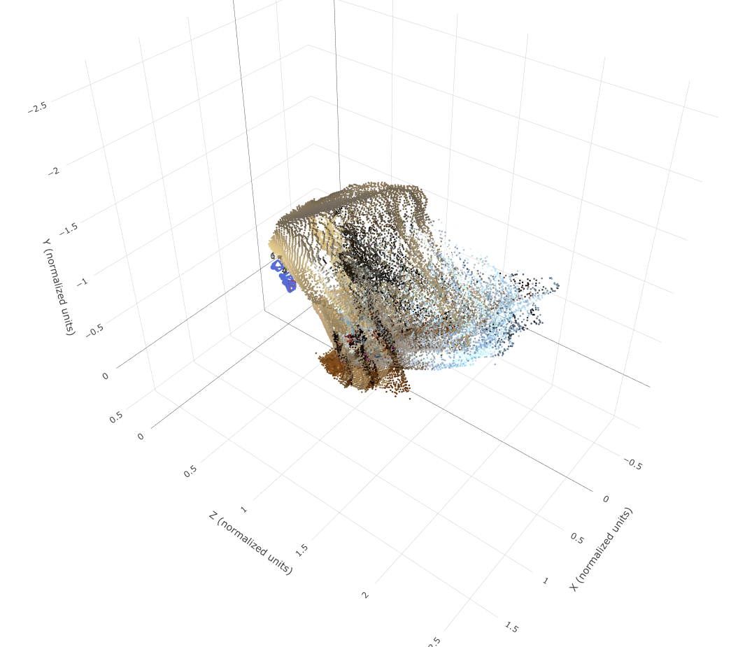
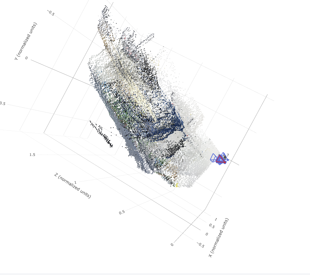
Comparisons of four different scenes are shown below, with the ground truth scene on the left, and the predicted geometry on the right.
| GT Image | Predicted Image |
|---|---|
 |
 |
 |
 |
 |
 |
 |
 |
To compensate for my laptop’s limited GPU, I used a batch size of 4 instead of 16, and only trained for 250 epochs instead of 1000, resulting in the slightly worse prediction views and loss curves than the TA’s example. I also decreased the learning rate to 0.0003.
As we can see in the metrics for the validation set vs. the test set, the test set performed slightly worse, with a higher depth abs rel, and a lower value for depth δ1 and translation / joint pose AUC at 30°. It did, however, perform better in terms of rotation AUC at 30° (higher value). Visually, the held-out scenes seemed to have more texture-less walls and a worse depth scale prediction of the room / scene itself.
I investigated the direct point-map direction. That is, I implemented a direct point map prediction head and loss function to investigate if it improved upon the existing network and training pipeline. For training, I used the same settings as before, and ran it on the same compute system (my laptop).
The final loss, after 250 epochs, converged to a value of 1.900, which is higher (i.e. worse) than the loss that the original method converged to at 1.424. This difference is visualized when comparing the loss curve below to the one shown above in section 3.2.

Comparison of Key Metrics
I compared some key metrics of the test (held-out) dataset with and without the direct prediction head. The results are as follows:
| Without | With | |
|---|---|---|
| Depth AbsRel | 0.183 | 0.184 |
| Depth δ1 | 0.00 | 0.737 |
| Rotation AUC 30° | 0.605 | 0.616 |
| Translation AUC 30° | 0.115 | 0.131 |
| Joint Pose AUC 30° | 0.097 | 0.110 |
This shows that the depth estimation was better with the direction prediction head (higher bas rel, lower δ1), but the rotation, translation, and joint pose aspects of the prediction all worsened.
Additionally, the translation error decreased from 49 degrees with the baseline (Task 3.2) method to 46 degrees with the new direct point head.
Scene comparison
The comparisons of four different scenes are shown below, with depth and camera based scene prediction on the left, and the direct point head prediction on the right.
| Depth and camera Image | Point head prediction Image |
|---|---|
 |
 |
 |
 |
 |
 |
 |
 |
The visualizations show that the improvement with the new prediction head is minor. Additionally, it should be noted that the loss values cannot be directly compared since the point prediction has an additional loss term added, so it’s loss will naturally be larger.