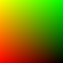

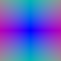

I implemented both the get_pixels_from_image and
get_rays_from_pixels methods. The following shows the
generated images on the left, as well as the TA (ground truth) images on
the right. They look identical.
I implemented the point sampling, which uniformly samples distances along each ray between near and far. The following shows the generated image on the left, and the TA (ground truth) image on the right.
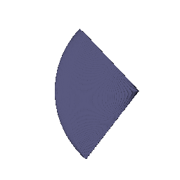
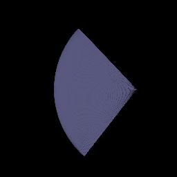
I implemented the volume rendering with the equations as described in the README. Below is the results, with the generated gif / depth image on the left, and the TA gif / depth image on the right. They’re both identical.
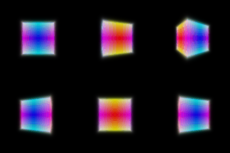

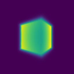

I implemented the random ray sampling, and used mean squared error (MSE) as the loss function to optimize over. The generated GIFs look identical.
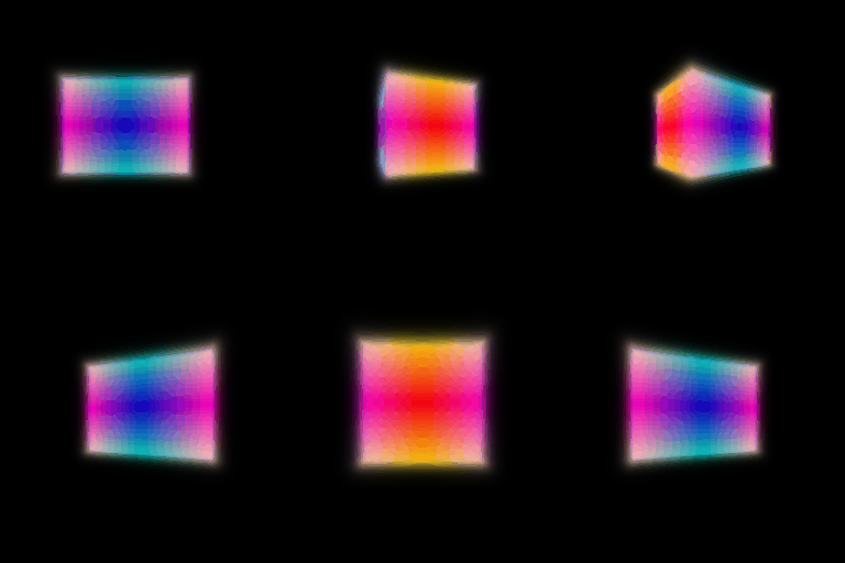
The training loss reached 0.000001. The outputted
box center was (0.25022992, 0.25057563, -0.00047936), and
the outputted box side lengths were
(2.00510740, 1.50358164, 1.50332522). The generated GIF
(left) looks identical to the TA GIF (right).

The NeRF model was optimized over the 128x128 images for 250 epochs. The final loss after training was TODO. Below is the resulting render for the lego bulldozer on the left, as well as the reference TA image on the right. They look nearly identical.


I implemented the view dependence into the model and ran the NeRF on the materials scene, with and without view dependence. Shown below, on the left is no view dependence, and on the right is with view dependence.
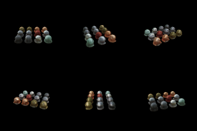

In the view dependence GIF, you can see that the materials appear to be more shiny, since the lighting varies per direction rather than being constant. In general, increased view dependence allows for a larger capacity to incorporate direction, rather than just geometry, into the learning for each image. However, this could result in overfitting when only a few views are available, thus reducing generalization quality. NeRF adds in direction late, so that density doesn’t depend on it, but color does, to mitigate this effect.
I implemented the SDF to volume density conversion function, and extended the NeuralSurface class to predict color. With this, I generated the following lego bulldozer model with the geometry (left) and the final render (right).
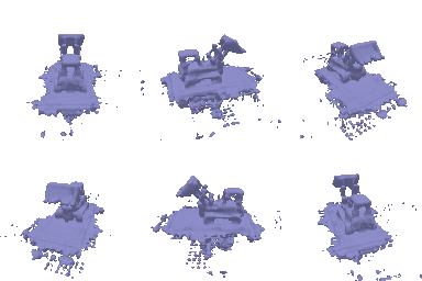
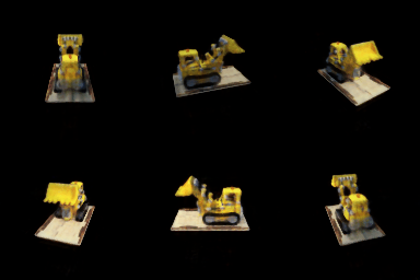
I used a beta value of 0.05, alpha value of 10.0, and an eikonal weight of 0.02, as this performed best, to generate the above results. I tried several other values of beta, alpha, and eikonal, but they all seemed to worsen the geometry, rather than improve it. All training was done for 250 epochs. The final loss after training for 250 epochs was 0.006376.
In general, a high beta value results in a smoother yet
blurrier image, whereas a smaller beta results in a sharper
but potentially noisier image with gradients mostly near the surface. An
SDF would be easier to train with higher
beta because the loss would be smoother and less
sensitive to sample placement. You would be likelier to learn an
accurate surface with a low beta because
the density is more concentrated on the true level set.
Tasks 5.1 / 5.2 - Unit tests pass: After
implementing parts 5.1 and 5.2, I ran
python unit_test_gaussians.py and validated that the 4 unit
tests passed: [4/4] Tests Passed.
Then, I ran python render.py to generate the GIF render.
The rendering took 14 minutes on my laptop GPU to render the 32 frame
GIF. The following GIF was rendered:
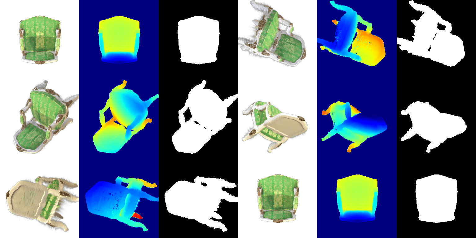
Since the reference image was of a still frame, I found the generated version of that still frame (frame 29), and created a side-by-side comparison, which is visualized below (generated on top, reference image below). They look near identical:
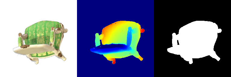
I implemented part 6 and ran the training pipeline on the truck data. The training ran for 1000 iterations and converged to a loss of 0.011. The mean PSNR was 29.806, and the mean SSIM was 0.943. The learning rates that I chose for the parameters, as present in the code, were as follows: - Opacities: 5e-2 - Scales: 5e-3 - Colours: 1e-2 - Means: 1e-3
These values were chosen since opacities and colours seem to converge fast, and so higher learning rates can be used, whereas means require a lower learning rate to avoid destroying important information (which could happen from a high learning rate resulting in a large optimizer step).
The generated training progress GIFs, as well as the final render GIF, are shown below.
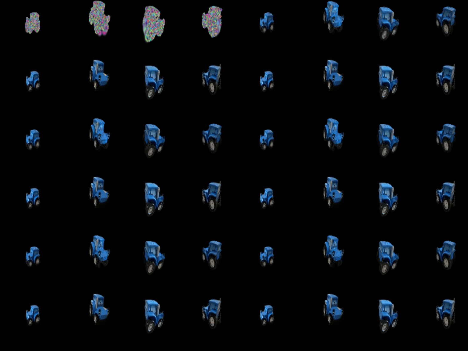

The reference images for the training and final render that were provided are shown below. The GIFs (above) seem to match up with the reference images (below).


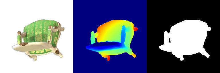
I implemented the spherical harmonics as described in the README. I then reran it using the spherical harmonics, and obtained the following GIF. On the top is the GIF with spherical harmonics (Q 7.1) and on the bottom is the GIF without (Q 5.5).
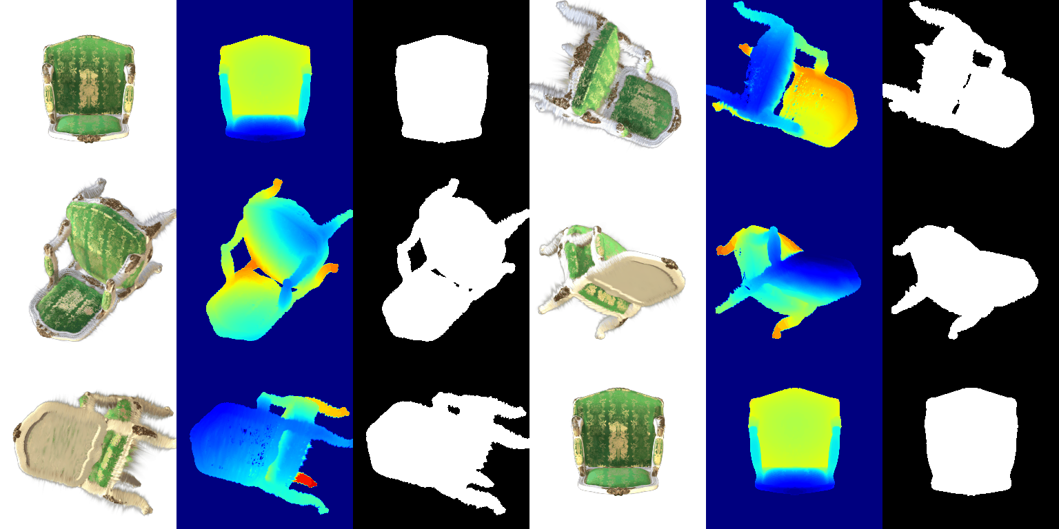
Below are some side-by-side frame comparisons. For each comparison, the spherical-harmonic variant is on top, and the older variant is on the bottom. Each comparison is followed by a description.

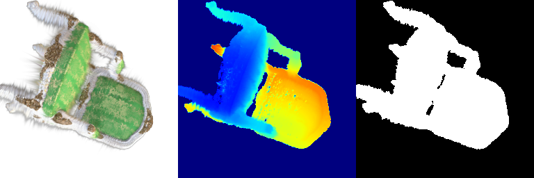
In the RGB images for these frames, you can see that the frame with spherical harmonics shows the brown and green parts of the chair as sharper and more contrastive.
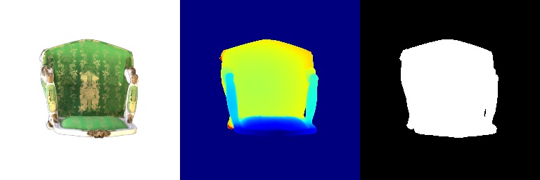
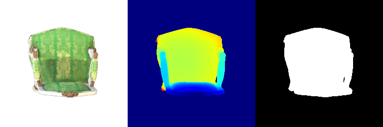
Here, you can once again see that the gold, brown, and green parts of the frame with spherical harmonicsare more contrastive. Additionally, you can see that the shading on the chair is view dependent rather than being a constant.