
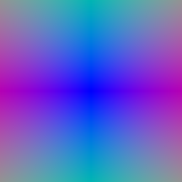
Both outputs match the TA output:
| xy_grid | rays |
|---|---|
|
|
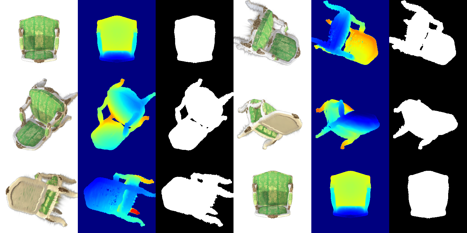
Samples from the first camera are visualized here below.
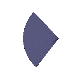
Depth are normalized by its maximum value.
| Rendering | Depth |
|---|---|
 |
 |
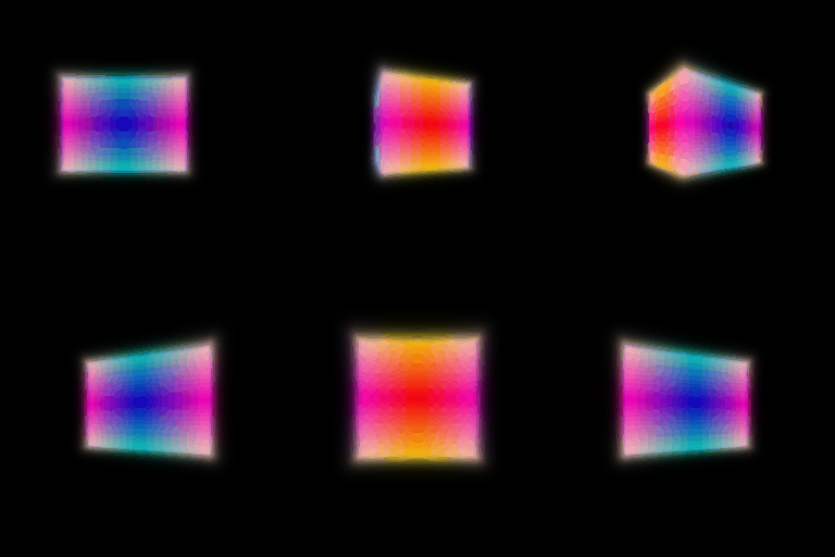
The box centre and side lengths after optimization:
Centre: (0.25, 0.25, 0.00), Side lengths: (2.01, 1.50, 1.50)
The resulting rectangular box rendering matches the TA reference.
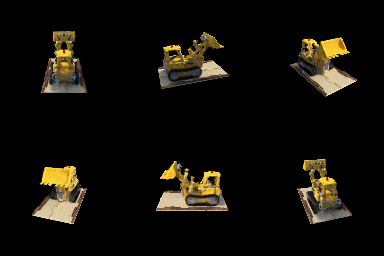
Results on the test set:
PSNR: 24.1958 dB; SSIM: 0.8836.
I implemented a six-layer MLP with 128 hidden units, ReLU density output, and Sigmoid RGB output. The visualization is as follows:
Modification on top of Part 3: I added a color network that takes the viewing direction as an additional input. The position network (adapted from Part 3) predicts density and features. The color network combines these features with the encoded viewing direction to predict color.
I compared this view-dependent approach with the original view-independent NeRF from Part 3 on the Materials scene. The results are as follows:
| NeRF model | Test PSNR (dB) | Test SSIM | gif rendering |
|---|---|---|---|
| Position only | 23.0487 | 0.8470 |  |
| Position + direction | 23.6961 | 0.8613 |  |
Adding view dependence increases PSNR by 0.6474 dB and SSIM by 0.0143, showing some improvement. In the renderings, we can also see brighter regions on some materials.
The trade-offs between increased view dependence and generalization quality are as follows: Increased view dependence can better represent areas with reflections and specular highlights (non-diffuse effects). However, excessive view dependence could cause the model to memorize and overfit to training views, thereby degrading generalization to unseen viewpoints. The current results do not show degraded novel-view generalization performance.
My coarse/fine sampling strategy is as follows: The coarse network evaluates 128 uniform samples and produces a sampling distribution, and 128 additional depths are sampled accordingly and merged with the coarse samples. A separate fine network evaluates all 256 points. Both networks are supervised with MSE loss on rendered images vs. ground-truth images.
| NeRF model | Test PSNR (dB) | Test SSIM | Training iters/s |
|---|---|---|---|
| w/o Coarse/fine sampling (Part 3) | 24.1958 | 0.8836 | 139.32 |
| w/ Coarse/fine sampling (Part 4.2) | 24.5522 | 0.8884 | 53.46 |
Visualization of the results from Coarse/fine sampling:

With coarse/fine sampling, PSNR improves by 0.3564 dB and SSIM by 0.0048, and training iterations take approximately 2.6× longer. Coarse/fine sampling uses 384 network queries per ray, compared with 128 queries for the baseline method.
Training configuration: alpha=10, beta=0.05, Eikonal weight 0.02, learning rate 5e-4, and 250 epochs on Lego images.
Results on the test set:
PSNR: 21.0314 dB; SSIM: 0.7552.
| Color | Extracted geometry |
|---|---|
 |
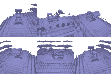 |
The main vehicle is recognizable. However, the extracted surface contains floating artifacts and "overlapped" layers.
Results of changing beta:
| Beta | Mean PSNR (dB) | Mean SSIM |
|---|---|---|
0.02 | 20.9064 | 0.7946 |
0.05 | 21.1654 | 0.7603 |
0.10 | 17.5059 | 0.5596 |
This comparison is done by rendering the previously trained epoch-200 checkpoint with different beta values, and the results are averaged over the first five validation views.
beta=0.05 has the highest PSNR and the relative high SSIM in this comparison, which supports my chosen setting.
Explanation of alpha and beta:
alpha defines the interior density and affects the opacity scale. beta controls the width of the transition from exterior to interior density.
A GIF rendering visualization is as follows:
Final selected learning rate:
| Parameter | Selected learning rate |
|---|---|
| Position | 1e-4 |
| Scale | 5e-3 |
| Opacity | 5e-3 |
| Color | 5e-3 |
A smaller learning rate for position can prevent the drifting of the gaussians.
Comparison on the learning rate of color:
| Color learning rate | Test PSNR (dB) | Test SSIM |
|---|---|---|
1e-3 | 26.890 | 0.898 |
5e-3 | 28.906 | 0.927 |
Both experiments were trained for 1,000 iterations.
The final run yields clearer windows and wheels in the visualization.
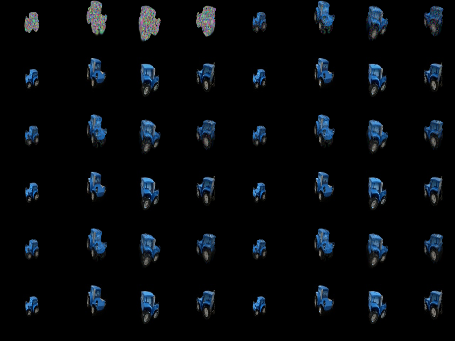

| Only DC spherical harmonic components (Part 5.5) | All spherical harmonics components (Part 7.1) |
|---|---|
|
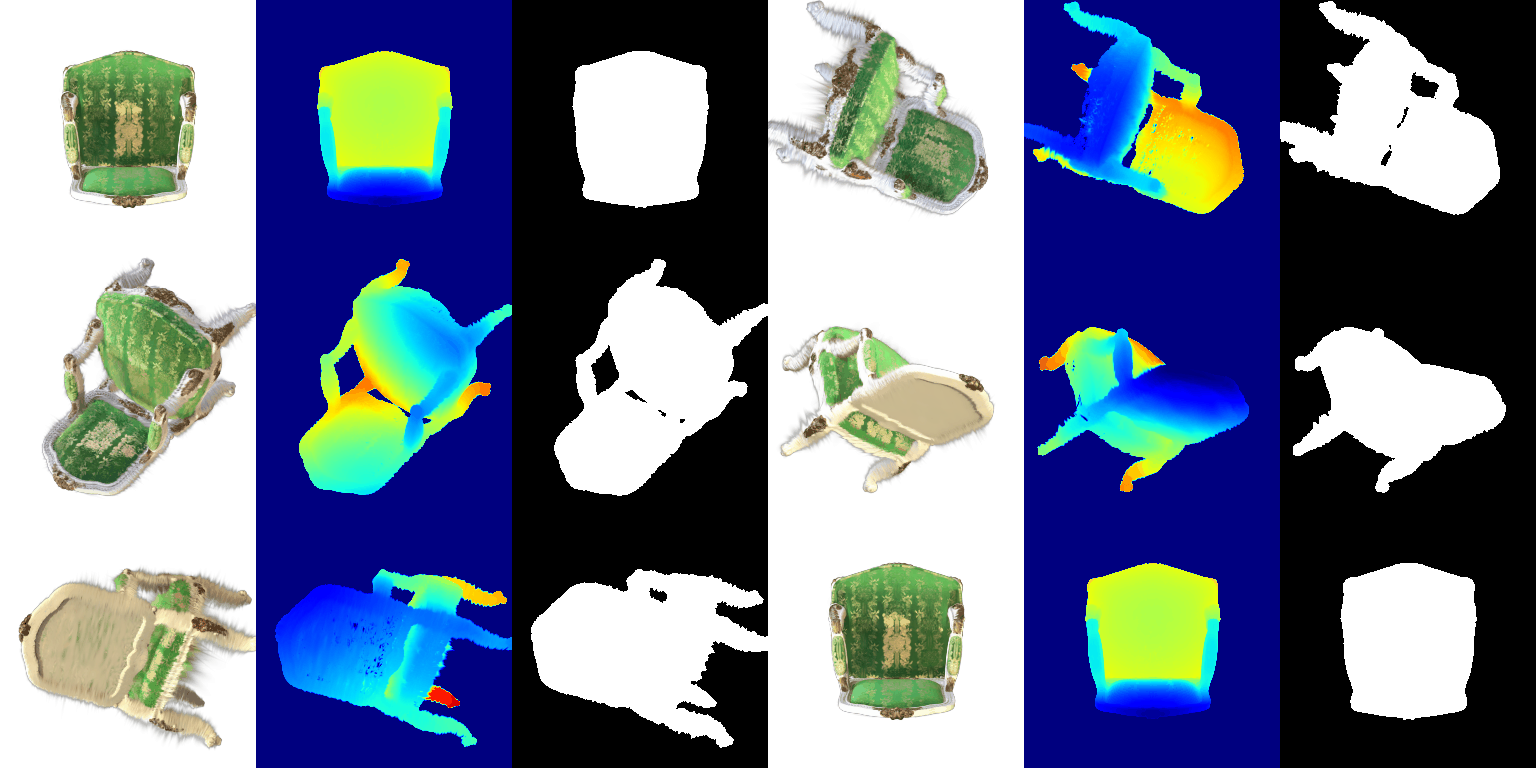 |
| Image | Only DC | Full SH | |
|---|---|---|---|
| 0 |  |
 |
The backrest appears to be darker and clearer with full SH, with the gold patterns more distinct to notice. The gold patterns could be more specular and shiny, so it may be better captured with view-dependent full SH. |
| 9 | 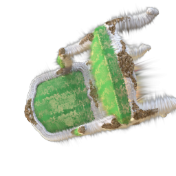 |
 |
The backrest and cushion are darker and more clearly defined with full SH. |
| 12 | 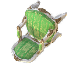 |
 |
The cushion looks darker and its gold pattern has stronger contrast with full SH. The backrest also shows clearer shading variations. |