
Left: optimized. Right: ground truth.
Left: optimized. Right: ground truth.
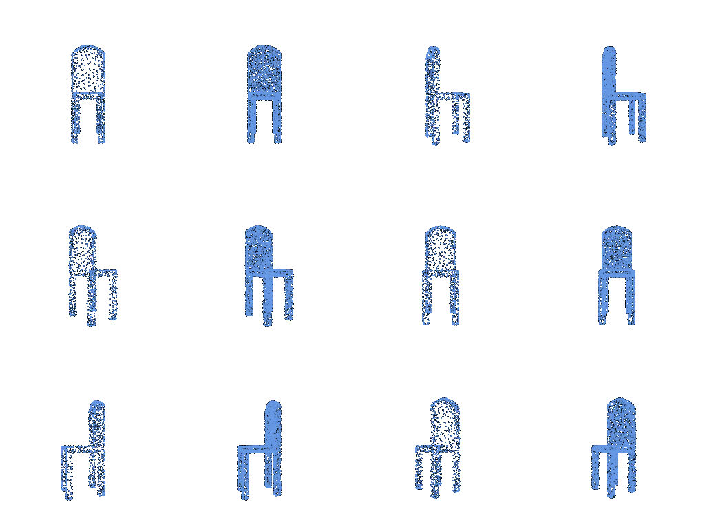
Left: optimized. Right: ground truth.

Model index is the zero-based object index in the test dataset.
Three examples from the test set:
| Model index | View | Input RGB | Prediction | Ground truth |
|---|---|---|---|---|
| 0 | 4 | 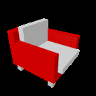 |
 |
 |
| 500 | 0 |  |
 |
 |
| 600 | 9 | 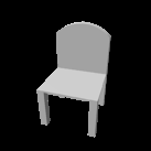 |
 |
 |
F1@0.05 = 75.32.

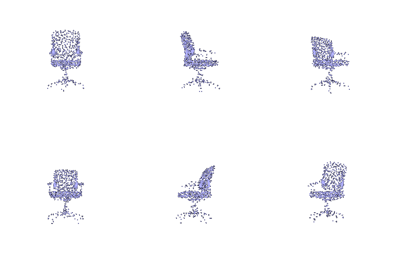
Three examples from the test set:
| Model index | View | Input RGB | Prediction | Ground truth |
|---|---|---|---|---|
| 350 | 0 |  |
 |
 |
| 500 | 0 | 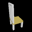 |
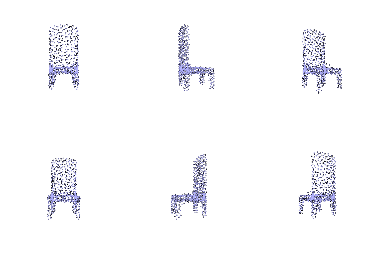 |
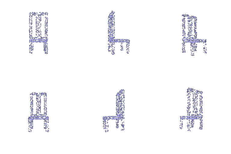 |
| 650 | 1 | 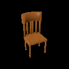 |
 |
 |
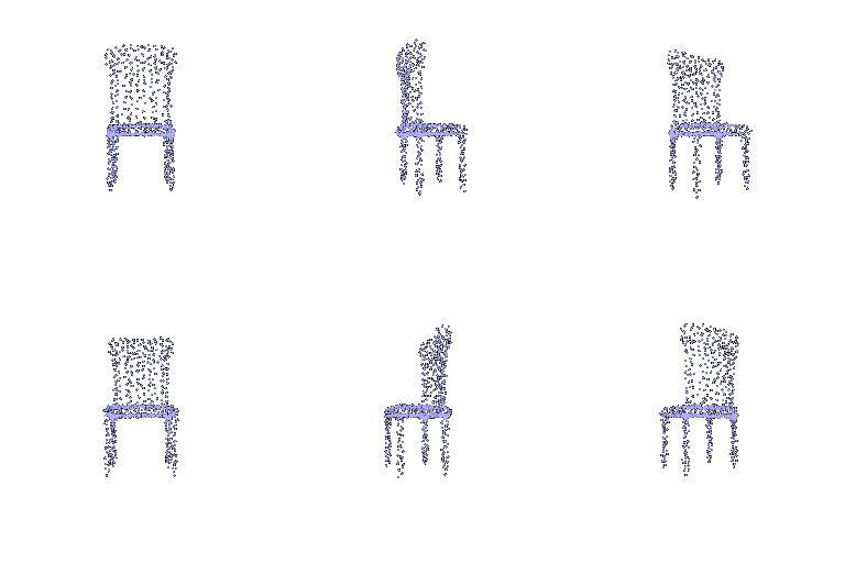
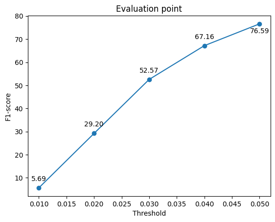
F1@0.05 = 76.59.
Three examples from the test set:
| Model index | View | Input RGB | Prediction | Ground truth |
|---|---|---|---|---|
| 250 | 0 |  |
 |
 |
| 550 | 8 |  |
 |
 |
| 600 | 5 | 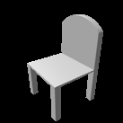 |
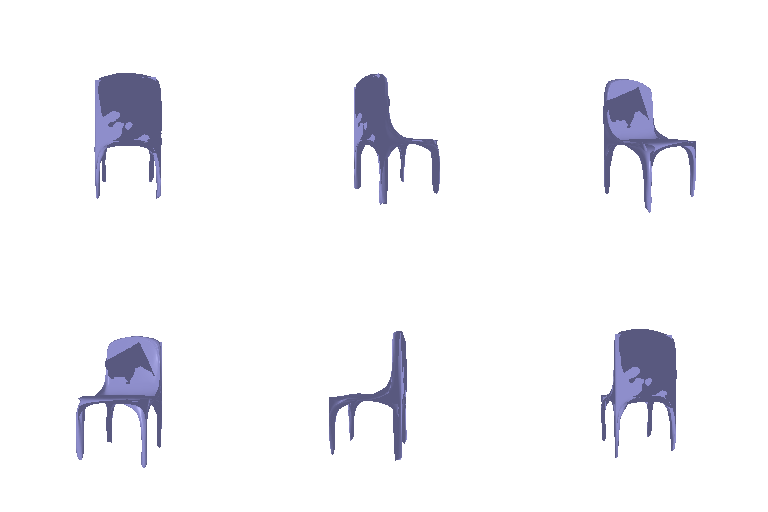 |
 |
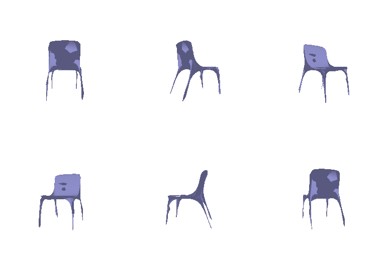
F1@0.05 = 73.15.
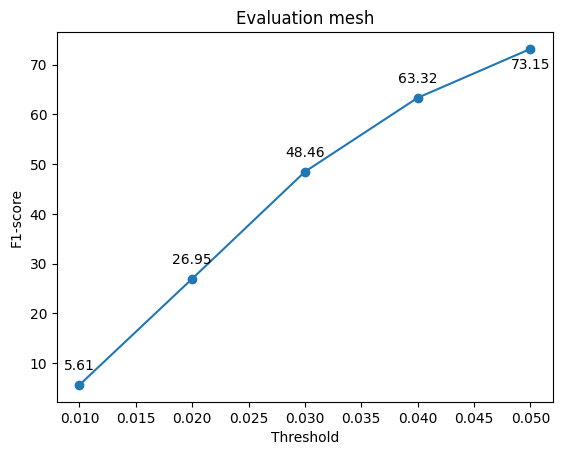
Compare the F1 score for meshes vs pointcloud vs voxel grids:
Point clouds achieve the highest F1@0.05 score (76.59), followed by voxel grids (75.32) and meshes (73.15).
Explanation:
Point clouds have no fixed connectivity, so they can represent disconnected components. Voxel grids can also represent disconnected parts and holes. Many chairs in the dataset have holes or cutouts in their backrests. Since the mesh model deforms a fixed-topology sphere, it may have difficulty reconstructing these disconnected 3D parts. This could explain the lower F1 score of the mesh prediction, compared with point cloud and voxel grid prediction.
Point clouds can also represent thin structures and fine details that may be lost in voxel grids. The voxel predictions are limited to a certain resolution. The resolution used here (32**3) could be insufficient for thin chair legs or small geometric details. This could explain that the point-cloud prediction yields a higher F1 score than voxel prediction.
The mesh model is compared with w_smooth = 0.01, 0.1 (default), and 1.
| w_smooth | Experiment | F1@0.05 | F1 plot |
|---|---|---|---|
| 0.01 | mesh_smooth001 |
74.50 |  |
| 0.1 | mesh_run1 |
73.15 |  |
| 1 | mesh_smooth1 |
72.23 |  |
The same three objects and input views as in 2.3 are used below.
| Model index | View | Input RGB | w_smooth = 0.01 | w_smooth = 0.1 | w_smooth = 1 | Ground truth |
|---|---|---|---|---|---|---|
| 250 | 0 | |
 |
|
 |
|
| 550 | 8 | |
 |
|
 |
|
| 600 | 5 | |
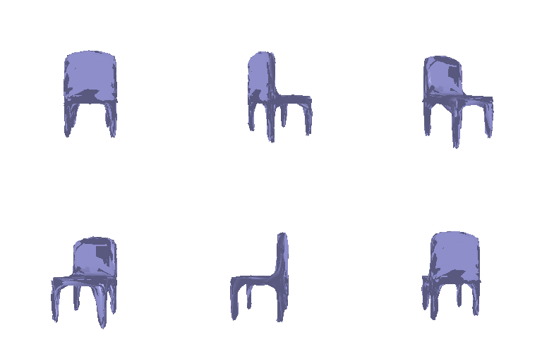 |
|
 |
|
Increasing w_smooth penalizes local surface irregularities more aggresively, encouraging smoother surfaces but potentially reducing geometric detail.
With low w_smooth (e.g. 0.01), the predictions contain more irregular surfaces but have better overall geometric resemblance.
When w_smooth = 1, the surfaces are smoother but some thin structures and geometric details are reduced.
Among these experiments, 0.01 yields the highest F1@0.05 (74.50), compared with 73.15 for 0.1 and 72.23 for 1.
For each comparison, the trained model and the tested 3D object are fixed, while only the input RGB viewpoint changes. All predictions use the same camera rendering pipeline.
Comparison 1: mesh model.
| View | Input RGB | Prediction | Ground truth | F1@0.05 |
|---|---|---|---|---|
| 0 |  |
 |
 |
66.99 |
| 1 |  |
 |
 |
55.78 |
| 2 | 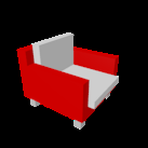 |
 |
 |
72.95 |
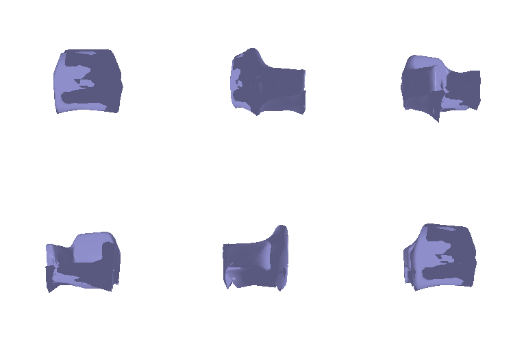
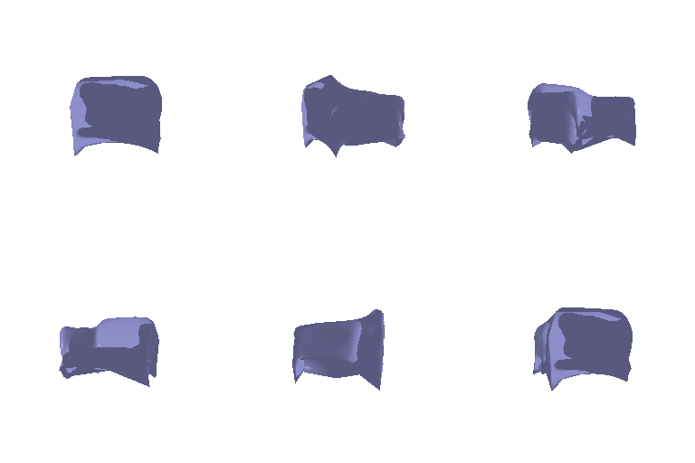
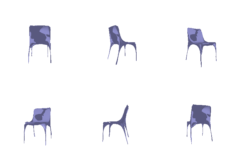
View 1 shows the chair from behind, hiding the seat and front legs. Its F1@0.05 is 55.78, lower than 66.99 for view 0 and 72.95 for view 2. Strong self-occlusion may correlate with low F1@0.05.
Comparison 2: mesh model.
| View | Input RGB | Prediction | Ground truth | F1@0.05 |
|---|---|---|---|---|
| 4 | 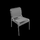 |
 |
 |
88.92 |
| 5 | 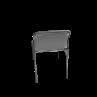 |
 |
 |
62.01 |
| 6 | 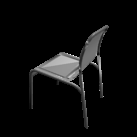 |
 |
 |
88.24 |
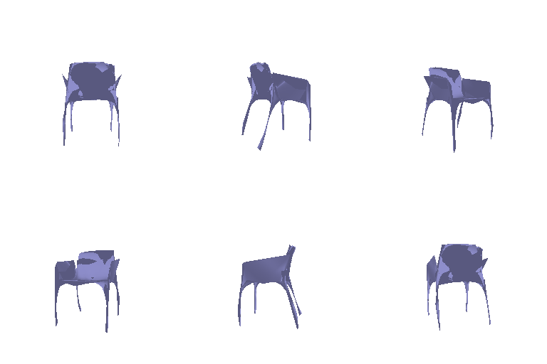
The rear-facing view 5 hides much of the seat and has F1@0.05 = 62.01. Views 4 and 6 expose more of the seat and score 88.92 and 88.24. The predictions differ in the seat and leg geometry.
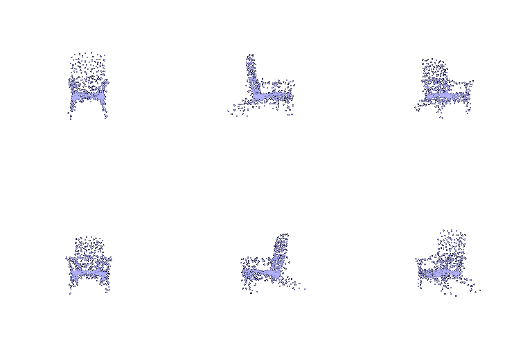
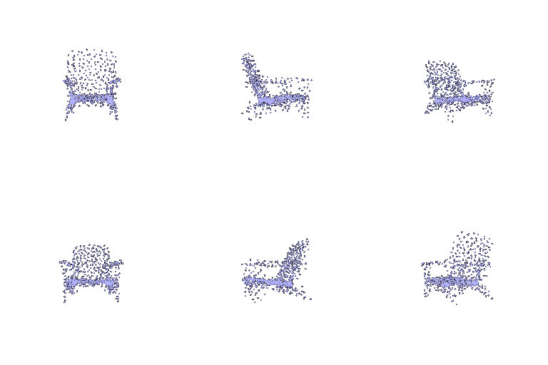
Comparison 3: point cloud model.
| View | Input RGB | Prediction | Ground truth | F1@0.05 |
|---|---|---|---|---|
| 4 | 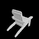 |
 |
 |
96.49 |
| 5 | 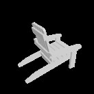 |
 |
 |
93.87 |
| 6 | 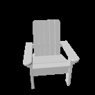 |
 |
 |
85.93 |
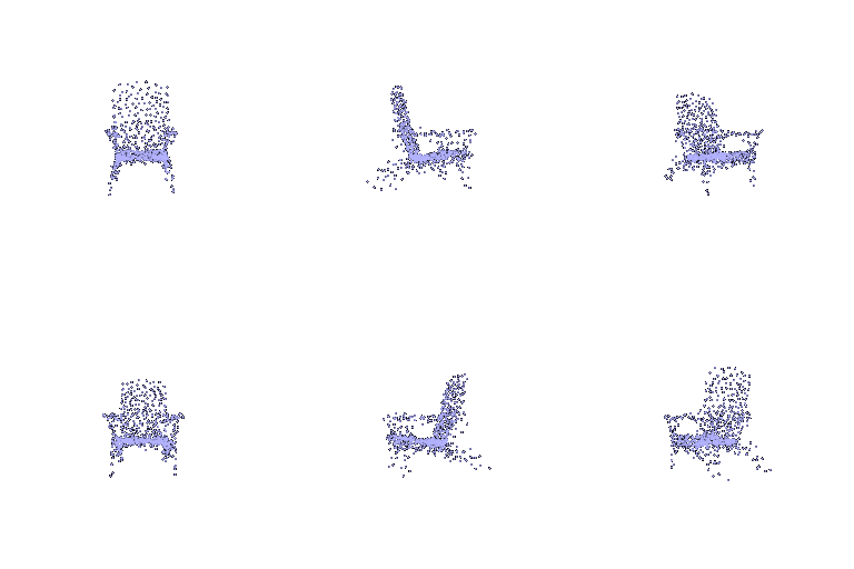
In view 6, the frontal input causes the legs and armrests to overlap in the image. Its F1@0.05 is 85.93, compared with 96.49 and 93.87 for views 4 and 5. The predicted leg structure is less consistent with the ground truth.
These examples show that strong self-occlusion may correlate with low F1@0.05, and good reconstruction may depend on the input viewpoint. The comparisons do not isolate occlusion from other viewpoint changes.
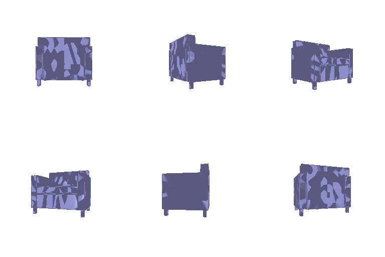
The decoder concatenates the 512-dim image feature with each 3D coordinate on a 32 × 32 × 32 grid in [-1, 1]³. An MLP (515 → 256 → 64 → 32 → 1, with ReLU) predicts an occupancy logit at each location. Training uses binary cross-entropy with logits; evaluation applies sigmoid and extracts the 0.5 isosurface.
| Model index | View | Input RGB | Prediction | Ground truth |
|---|---|---|---|---|
| 0 | 2 | 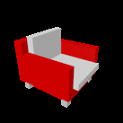 |
 |
 |
| 550 | 0 | 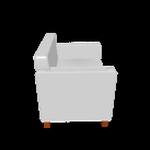 |
 |
 |
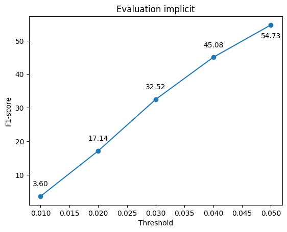
F1@0.05 = 54.73.
The coordinate-conditioned MLP scores lower than the convolutional voxel decoder in these runs (54.73 vs. 75.32).
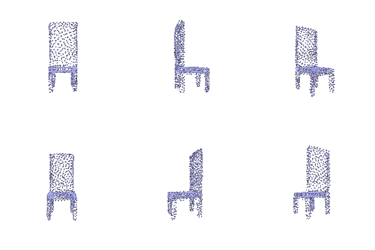
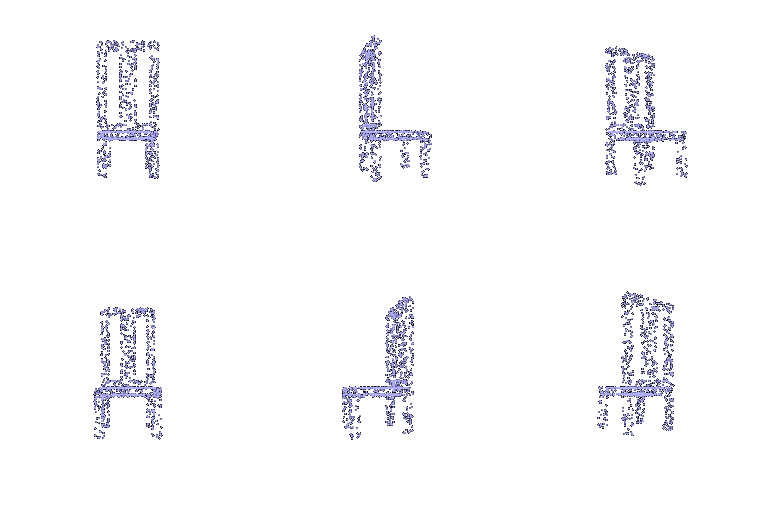
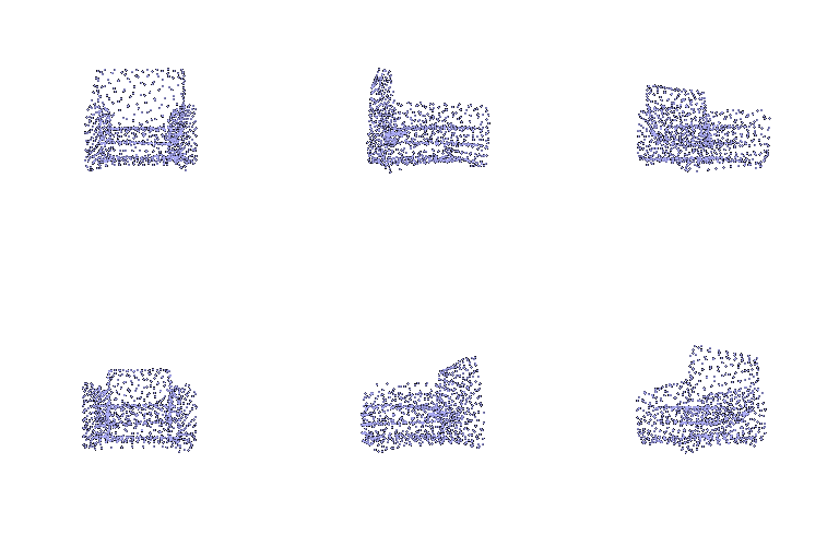
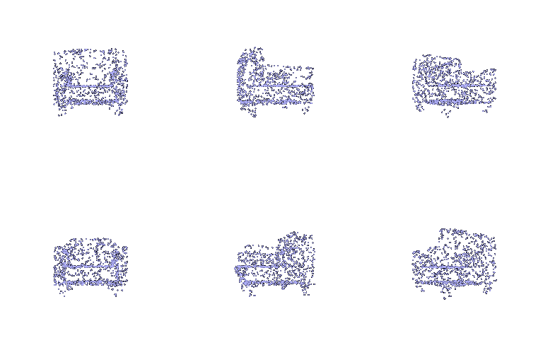
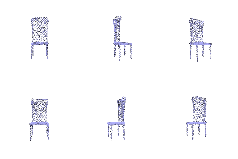
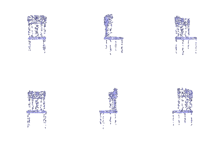
The decoder uses four independent surface patches. Each patch concatenates a 512-dim image feature with a 2D coordinate from a 16 × 16 grid in [0, 1]². An MLP (514 → 256 → 128 → 64 → 3, with ReLU between hidden layers) maps each coordinate to a 3D point. The four patches produce 1,024 points in total and are trained with Chamfer loss.
| Model index | View | Input RGB | Prediction | Ground truth |
|---|---|---|---|---|
| 500 | 5 |  |
 |
 |
| 0 | 4 | 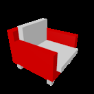 |
 |
 |
| 650 | 2 | 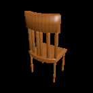 |
 |
 |
F1@0.05 = 75.51.
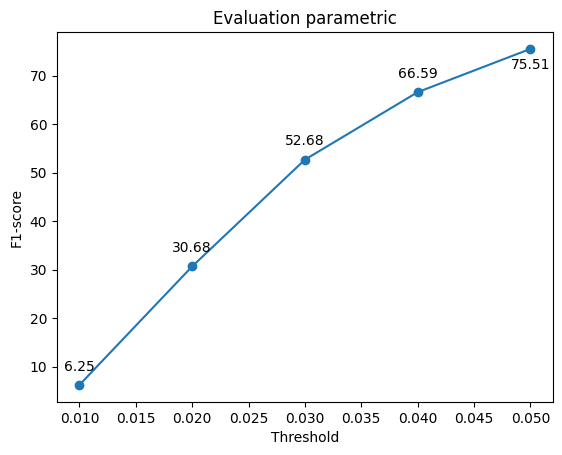
The selected predictions recover the main chair structures, with remaining differences in thin parts and surface detail. The patch-based decoder achieves a similar F1@0.05 to the direct point-cloud decoder (75.51 vs. 76.59).