

Depth is unprojected per view using the resized intrinsics and the world camera pose. Pixels are lifted to camera space with K-1, scaled by the z-depth, and transformed to world space with R·p + t. Visualized below in the original world frame (meters), before canonicalization.
All cameras and points are re-expressed in camera 0's frame (Trel = Tworld_from_ref-1 Tworld_from_cam, so camera 0 becomes identity), then divided by the shared scene scale (the valid-point centroid's distance from the origin), so the centroid sits at distance 1. Translations, depth and points are all scaled, never re-centered.


For 1.4, each pixel's camera-space direction (K-1[u, v, 1]T) is rotated into the canonical world frame by the pose rotation and normalized to a unit vector, and the ray origin is the camera center broadcast to every pixel. For 1.5, each ray is written as Plücker coordinates [d, m], with direction d and moment m = o × d. Together, [d, m] give a minimal, translation-aware 6-channel encoding of a ray's full 3D line, independent of image resolution.
d alone only encodes a ray's orientation, so two parallel rays through different points in space would look identical. The moment m fills that gap, it is zero only for rays through the origin, and its magnitude is the perpendicular distance from the origin to the ray, so it encodes where the ray actually sits in space. Together [d, m] fully specify the ray as a compact, resolution-independent camera-conditioning signal.Reprojection error stays well under the 0.01 px requirement, and the valid-point centroid distance is 1.0 for every sampled scene, confirming the Q1.2/Q1.3 implementations are consistent (check_data.py).
{
  "split": "train",
  "dataset_samples": 224,
  "checked_samples": 4,
  "samples": [
    {
      "sequence_name": "e050c15a8d_frame_007080",
      "views": 8, "resolution": 224,
      "valid_depth_fraction": 0.9779,
      "max_reprojection_error_px": 0.000113,
      "max_ray_reprojection_error_px": 0.000109,
      "centroid_distance": 1.0
    },
    {
      "sequence_name": "5f99900f09_frame_002820",
      "views": 8, "resolution": 224,
      "valid_depth_fraction": 0.9903,
      "max_reprojection_error_px": 0.000123,
      "max_ray_reprojection_error_px": 0.000111,
      "centroid_distance": 0.99999994
    },
    {
      "sequence_name": "47b37eb6f9_frame_002720",
      "views": 8, "resolution": 224,
      "valid_depth_fraction": 0.9610,
      "max_reprojection_error_px": 0.0000988,
      "max_ray_reprojection_error_px": 0.0000890,
      "centroid_distance": 1.0
    },
    {
      "sequence_name": "4c5c60fa76_frame_006690",
      "views": 8, "resolution": 224,
      "valid_depth_fraction": 0.7517,
      "max_reprojection_error_px": 0.000116,
      "max_ray_reprojection_error_px": 0.000107,
      "centroid_distance": 1.0
    }
  ],
  "batch_shapes": {
    "rgb": [2, 8, 3, 224, 224], "depth": [2, 8, 1, 224, 224],
    "depth_valid": [2, 8, 1, 224, 224], "K": [2, 8, 3, 3],
    "T_world_from_camera": [2, 8, 4, 4], "scene_scale": [2],
    "points_world": [2, 8, 3, 224, 224],
    "ray_origins": [2, 8, 3, 224, 224], "ray_directions": [2, 8, 3, 224, 224],
    "plucker": [2, 8, 6, 224, 224]
  }
}
One fixed batch, 2000 steps, S = 2 source views (14.6M parameters). Final validation PSNR 30.88 dB (SSIM 0.869), loss 0.00088, comfortably above the 30 dB target.

val_epoch000.png. Columns are the 2 source views, ground truth and prediction, and rows are different samples. The overfit prediction nearly matches the ground truth.Settings. S = 2 source views, patch size 8, d_model 384, 8 transformer layers, head dim 64, QK-norm enabled, batch size 4, AdamW (lr 2e-4, weight decay 0.05, 200-step warmup), bfloat16 autocast, 100 epochs on the full training split (224×224, 8 views/scene, sampling range 32).


Evaluated best.pt on the validation split over the number of source views (1/2/4) and target-ray conditioning (correct uses the true target rays, shuffled swaps in another target view's rays, none zeroes the rays).
| Source views | Conditioning | PSNR | SSIM | Loss | # images |
|---|---|---|---|---|---|
| 1 | correct | 15.19 | 0.5583 | 0.0352 | 196 |
| 2 | correct | 16.13 | 0.5603 | 0.0294 | 168 |
| 4 | correct | 16.86 | 0.5754 | 0.0248 | 112 |
| 1 | shuffled | 11.80 | 0.4873 | 0.0730 | 196 |
| 2 | shuffled | 11.48 | 0.4721 | 0.0780 | 168 |
| 4 | shuffled | 11.58 | 0.4732 | 0.0784 | 112 |
| 1 | none | 12.47 | 0.5281 | 0.0589 | 196 |
| 2 | none | 12.44 | 0.5264 | 0.0592 | 168 |
| 4 | none | 12.46 | 0.5370 | 0.0588 | 112 |
Effect of source-view count, correct target rays throughout. Every panel is rendered at the same native 224×224 resolution, so the wider S=4 row is simply longer, not more compressed.

Effect of target-ray conditioning, fixed at S=2. Sources and ground truth are identical across the three conditioning settings, so the comparison isolates what the prediction column alone changes.

Discussion. More source views helps but only modestly (15.19, 16.13 and 16.86 dB PSNR for S=1, S=2 and S=4), since extra views mostly add redundant context the model already captures from the first view or two.
Ray conditioning matters far more, correct target rays beat the ablations by 2.7 to 5.3 dB PSNR, a gap that widens as S grows, confirming the model genuinely uses the target rays to select the queried viewpoint rather than guessing a generic view. SSIM moves the same way but less sharply (e.g. S=2, 0.560 correct vs. 0.472 shuffled vs. 0.526 none). The two failure modes also look qualitatively different in the combined figure above, none (zero rays) collapses to a flat, low-frequency color with no structure, the safe average under no directional signal, while shuffled confidently reconstructs real room geometry from the wrong camera pose, which is why it scores even lower than none despite looking more like a photo.
Hypothesis. Adding an LPIPS perceptual loss term will produce visually sharper predictions than MSE alone, at the cost of lower PSNR/SSIM, since perceptual losses are known to trade exact pixel match for higher-frequency, more plausible-looking detail. Trained with loss = MSE + 0.5·LPIPS, otherwise identical architecture (configs/lvsm_lpips.json, 100 epochs).

| Loss | Source views | PSNR | SSIM | MSE |
|---|---|---|---|---|
| MSE only (2.2) | 1 | 15.19 | 0.5583 | 0.0352 |
| MSE only (2.2) | 2 | 16.13 | 0.5603 | 0.0294 |
| MSE only (2.2) | 4 | 16.86 | 0.5754 | 0.0248 |
| MSE + 0.5·LPIPS | 1 | 14.33 | 0.4637 | 0.0401 |
| MSE + 0.5·LPIPS | 2 | 14.76 | 0.4563 | 0.0368 |
| MSE + 0.5·LPIPS | 4 | 14.99 | 0.4589 | 0.0342 |
Adding LPIPS costs about 1.3–1.9 dB PSNR and 0.10–0.12 SSIM at every source-view count, evaluated with correct target-ray conditioning.


The last column of each grid is the prediction. The MSE-only model is softer and more uniformly blurred, while the LPIPS model's predictions show a higher-frequency, patch-grained texture (visible as a repeating checkerboard-like pattern at the 8×8 patch scale) instead of a flat blur, since it is trying to hallucinate plausible texture rather than average over uncertainty, which raises perceptual detail but can disagree with the exact ground-truth pixels.
Rendered synthetic camera trajectories with scripts/lvsm_flythrough.py (interpolated path, S = 2), extrapolating past the source views where both models are under more stress. Drag the divider to compare the two training runs frame-by-frame on the same trajectory.
Clip 0, held-out PSNR 16.63 dB (MSE) vs. 14.52 dB (MSE+LPIPS)
Clip 2, held-out PSNR 16.38 dB (MSE) vs. 14.54 dB (MSE+LPIPS)
Answer. LPIPS does not improve PSNR/SSIM at any source-view count, it is strictly worse on both metrics, which matches the predicted cost. The sharpness side is more mixed, under extrapolation in the flythrough, the MSE-only model blurs under uncertainty while the LPIPS model paints a patch-scale texture that looks less blurry, but that texture does not actually line up with the true scene, so it reads as different rather than clearly better.
Model. Frozen DINOv2 ViT-B/14 encoder, 8 frame/global attention pairs (16 blocks, width 384, 6 heads), 4-block cross-view camera head, RGB-refined depth decoder. Fit to one fixed training clip for 40 epochs.

By epoch 40 the overfit clip reaches depth AbsRel 0.036, depth δ1 0.956, and near-perfect pose accuracy (rotation AUC@5°/15°/30° = 1.0, pose AUC@30° = 0.999).


The predicted point cloud and camera trajectory are visually indistinguishable from ground truth after overfitting, consistent with the near-1.0 rotation/pose AUCs above.
To localize the small remaining disagreement, each point is colored by its distance to the corresponding GT point (same pixel, turbo colormap, blue is low and red is high), rendered from the same camera pose as above. Drag the divider to slide between the predicted geometry and this error heatmap.
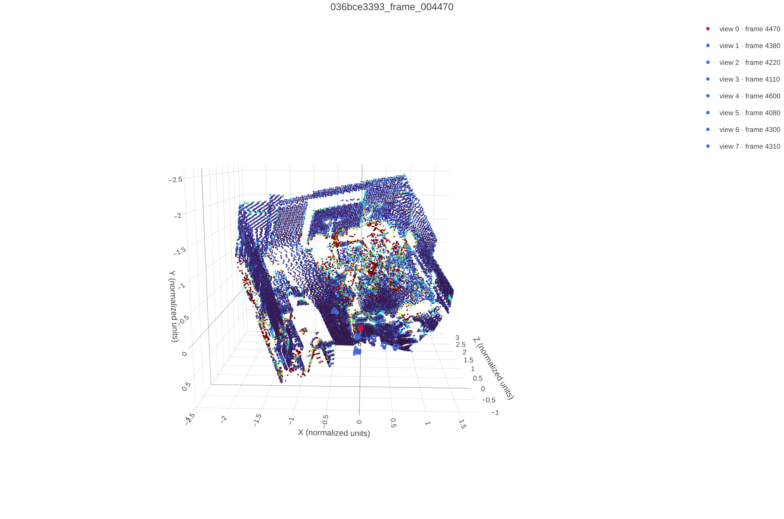
Per-point GT-prediction distance, mean 0.055, 95th percentile 0.299, max 1.625 (normalized units)
Settings. Same architecture as 3.1 (frozen DINOv2 ViT-B/14, 8 frame/global attention pairs, width 384, 6 heads), trained on the full ScanNet++ iPhone training split for 1000 epochs, 8 views per sample with sampling range 32, 224px images, batch size 16, learning rate 6e-4 with 10 warmup epochs decaying to a 5% floor, weight decay 0.01, loss weights camera 5.0 and depth 1.0 (configs/vggt.json).

Evaluated best.pt on the validation and test splits using 8 views from the first 32 prepared frames, 224px, seed 825.
| Split | Depth AbsRel | Depth δ1 | Rot. AUC@5°/15°/30° | Transl. AUC@5°/15°/30° | Joint AUC@5°/15°/30° |
|---|---|---|---|---|---|
| Validation | 0.148 | 0.824 | 0.210 / 0.536 / 0.709 | 0.013 / 0.078 / 0.184 | 0.003 / 0.063 / 0.160 |
| Test | 0.154 | 0.822 | 0.208 / 0.561 / 0.752 | 0.011 / 0.063 / 0.175 | 0.001 / 0.046 / 0.159 |
Depth recovers well (AbsRel around 0.15, δ1 around 0.82, close to the 3.1 overfit numbers), but camera pose is the bottleneck. Rotation is reasonably accurate (AUC@30° around 0.71-0.75) while translation direction is much harder (AUC@30° around 0.18), which drags the joint pose AUC down to around 0.16 at 30°.
The four scenes below show the same pattern visually, room shape and layout are reconstructed correctly from depth, but the predicted camera trajectory is more compressed and offset than the ground truth, consistent with translation being the weaker signal. Test slightly outperforms validation, so there is no sign of overfitting to the validation scenes.
Each widget below orbits the camera around the same ground-truth and predicted point cloud, synced frame for frame, for four different validation scenes. Drag a divider to compare.


Scene 09c1414f1b


Scene 21d970d8de


Scene 280b83fcf3


Scene 2b1dc6d6a5
Hypothesis. Evaluating the 3.2 model (trained with 8 views) using more views than it was trained with will improve depth and pose accuracy, since more observations give the attention blocks additional triangulation constraints, at the cost of runtime and memory that grow with the view count.
Settings. Same outputs/vggt_train/best.pt checkpoint as 3.2, no retraining. Varied only the number of views sampled at evaluation (2, 4, 8, 16, 32) from the same 32-frame prepared validation window, 224px, seed 825, batch size 4. Runtime is seconds per batch (best of 3 timed runs after a warmup pass) and memory is peak allocated GPU memory, both from scripts/vggt_view_scaling.py.

Answer. More views does not help, depth and translation accuracy are both best with the fewest views tested and get steadily worse as the view count grows. Rotation accuracy is the one exception, peaking right at the trained count of 8 views before declining either direction. Runtime and memory both grow with view count as predicted, but sub-linearly, since per-frame encoding and the depth/camera heads dominate over the quadratic cost of global attention at this scale. The accuracy drop suggests the model overfits to its training-time view count rather than learning a view-count-invariant triangulation rule, extra views add wider-baseline pairs the 8-view training distribution rarely saw, which the pose head handles worse, not better.
Follow-up. Is that really about harder pairs, or does the model just get worse at the same kind of pair once more views are added? Grouping pairs by frame-gap (a stand-in for baseline) and tracking each group separately across view counts answers this with scripts/vggt_pair_breakdown.py.

The pair mix barely shifts with view count, every bucket keeps roughly its same share throughout. What does shift is accuracy within a bucket, the middle baseline ranges get noticeably worse as more views are added, while the widest-baseline pairs were already near their ceiling and stay flat. So the earlier explanation was only half right, it is less that more views add harder pairs, and more that the model gets worse on the same kind of pair once more tokens compete for attention.