
xy_grid)
Pixel coordinates mapped to [−1, 1] (left) and the resulting ray directions shown as colour (right).
xy_grid)64 evenly spaced samples per ray between near (0) and far (5), for the first camera.

Weights are T·(1 − exp(−σΔt)). Colour and depth are the weighted sums, and depth is normalised by its maximum.

part_1.gif)
Trained for 1000 epochs with an MSE loss, batch size 4096 and learning rate 0.0005.
| x | y | z | |
|---|---|---|---|
| Box centre | 0.25 | 0.25 | 0.00 |
| Box side lengths | 2.01 | 1.50 | 1.50 |
Raw values: centre (0.2502303123474121, 0.2505737245082855, −0.00048422403051517904), side lengths (2.0051159858703613, 1.5035902261734009, 1.5033924579620361).

part_2.gif)Position-only MLP (6 layers of 128 units, skip at layer 3, 6 harmonic frequencies) trained on lego at 128×128 for 250 epochs, learning rate 0.0005.

Colour is now predicted by a small head that takes the position feature and the harmonic-encoded ray direction, while density stays a function of position only. Shown on the materials scene and on lego.


Discussion. Over the object pixels the two renders differ by about 14/255 on materials and 11/255 on lego. On materials the view-dependent model is about 16% darker on average (mean brightness 76 vs. 64) with deeper colours, whereas the position-only model gives lighter, greyer balls, consistent with averaging highlights and reflections into one colour per point. On lego the mean brightness is unchanged (111 vs. 111) and the difference is a fine speckle on edges and texture, as expected for a mostly diffuse scene. The two GIFs come from separate training runs, so part of the difference is run-to-run noise, and without held-out metrics I cannot say which generalises better.
Trade-offs. View dependence is needed for highlights and reflections, which a position-only model averages into one colour. The cost is overfitting: a direction-conditioned head can memorise per-view colours instead of fixing the geometry, which hurts unseen views. I limit this by keeping density position-only and encoding direction with few frequencies (2 vs. 6 for position). I did not measure generalisation on held-out views.
Coarse network on 64 evenly spaced samples. Its weights draw 64 more, and the fine network is evaluated on all 128 merged samples. Same materials settings as 4.1 otherwise.

Epoch 200, 30 of 100 validation views:
| Val PSNR | Render time | Parameters | |
|---|---|---|---|
| Plain NeRF (128 points/ray) | 23.70 dB | 185 ms/image | 102k |
| Coarse/fine (64 coarse + 64 fine) | 23.78 dB | 401 ms/image | 204k |
Discussion. No real quality gain (the 0.08 dB gap is within noise: random fine sampling, only 30 views) and about 2.2× slower to render, since each ray costs 64 coarse + 128 fine evaluations against 128, with twice the parameters.
Best run. α = 10, β = 0.05, eikonal weight 0.02, learning rate 0.0002 (decayed by 0.8 every 50 epochs), batch size 1024, 250 epochs, 128 samples per ray. The SDF is initialised as a sphere of radius 1.5 (distance = MLP output + ∥x∥ − 1.5, with a small-weight last layer), so training starts from a valid surface that encloses the object. The lower learning rate keeps that surface from collapsing early.


Bad run. With the default learning rate of 0.0005 the optimisation fails: the bulldozer never forms. The renders are almost black with a stray cloud near the bottom of the frame.

α and β. α is the density deep inside the object (how opaque it is). β is the width of the transition at the surface: a small β gives a near-step density, a large β a thick, smooth one.
Chair rendered with only the view-independent (DC) colour. Each frame shows RGB, depth and mask.

render.py)Isotropic Gaussians initialised from the truck point cloud, trained with an L1 loss.
| Parameter | Learning rate |
|---|---|
| Opacities (pre-activation) | 0.05 |
| Scales (pre-activation) | 0.001 |
| Colours | 0.01 |
| Means | 0.0001 |
1000 iterations. Evaluation on the held-out views: PSNR = 28.519, SSIM = 0.930.


Same frame, DC only (left) vs. spherical harmonics (right).

Frame 0. DC-only is lighter and flatter, with a washed-out gold pattern. With SH the green is deeper and the pattern has more contrast, since the fabric's sheen changes with view direction.

Frame 15. Same difference: SH gives darker greens and a sharper pattern. Geometry is identical, only colour changes.

Frame 24. The underside of the chair, where little fabric is visible. The two renders are nearly identical, with only slightly richer green under SH.
| Setup | PSNR | SSIM |
|---|---|---|
| Baseline (isotropic, L1, Q6 learning rates) | 16.260 | 0.622 |
| Improved | 22.703 | 0.828 |
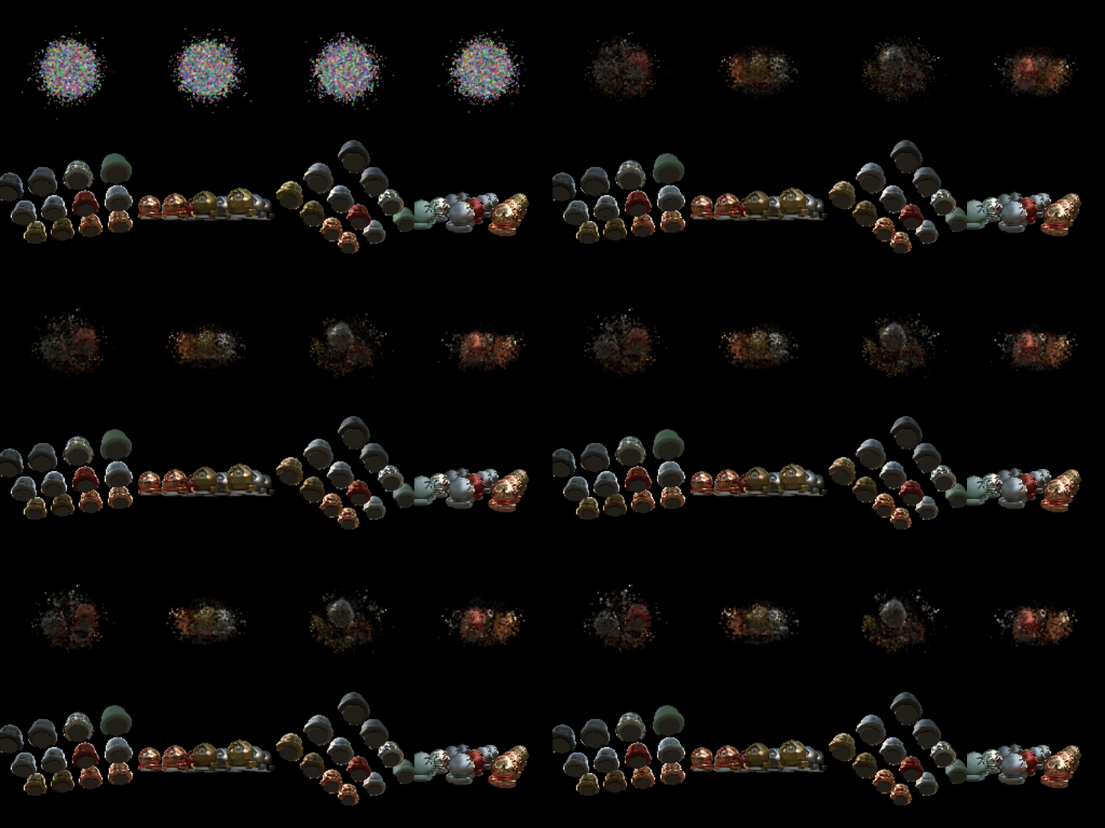


Comparison. The improved model gains 6.4 dB PSNR and 0.21 SSIM. By the end the baseline is still a dim, speckled blob, while the improved model places every ball in the right position with the right colour. It stays blurrier than the ground truth, with softer edges and weaker highlights on the metallic balls.
Modifications relative to Q6: