16-825 Assignment 4: Multi-View Transformers
Name: Ruinian (Ray) Xue
AndrewID: ruinianx
16-825 Assignment 4: Multi-View Transformers1. Multi-View Data Preprocessing (20 points)1.2. Depth UnprojectionScreenshot1.3. Camera and Depth CanonicalizationScreenshot1.7. Final Checkcheck_data.py outputDiscussionsCanonicalizationWorld-space ray directionsPlücker moment2. Novel-View Synthesis with Mini-LVSM (40 points)2.1. Overfitting (10 points)Overfit PSNROverfit visualization2.2. Training and Evaluation (30 points)Training curvesResults for ablation settingTraining visualizationsEpoch 0Epoch 50Epoch 95Evaluation visualizationsTraining settingsDiscussions2.3. Bonus: Analysis and Exploration (10 points)Question & Experimental settingResult & ConclusionVisualizationEpoch 0Epoch 50Epoch 95Explanation & Limitation3. Multi-View Geometry with Mini-VGGT (40 points)3.1. Overfitting (10 points)Loss curve imageScreenshot3.2. Training and Evaluation (30 points)Loss curve imageValidation/test metricsScreenshotTraining settingDiscussion
1. Multi-View Data Preprocessing (20 points)
1.2. Depth Unprojection
Implement unproject_depth to convert depth pixels into world-space 3D points using the supplied camera poses. Depth is optical-axis z-depth, not distance along a unit ray.
After Q1.1–1.2, visualize points and cameras in the original world frame (meters):
python scripts/visualize_data.py --stage unprojection --num-scenes 5 --max-points 10000 --output outputs/unprojectionScreenshot
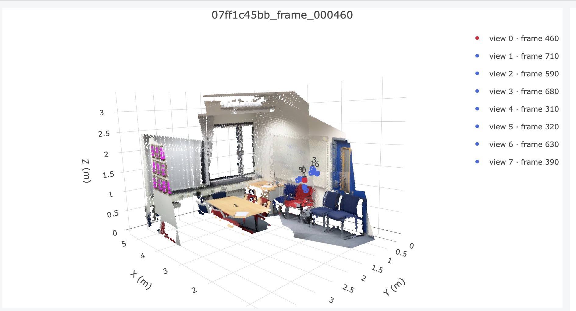
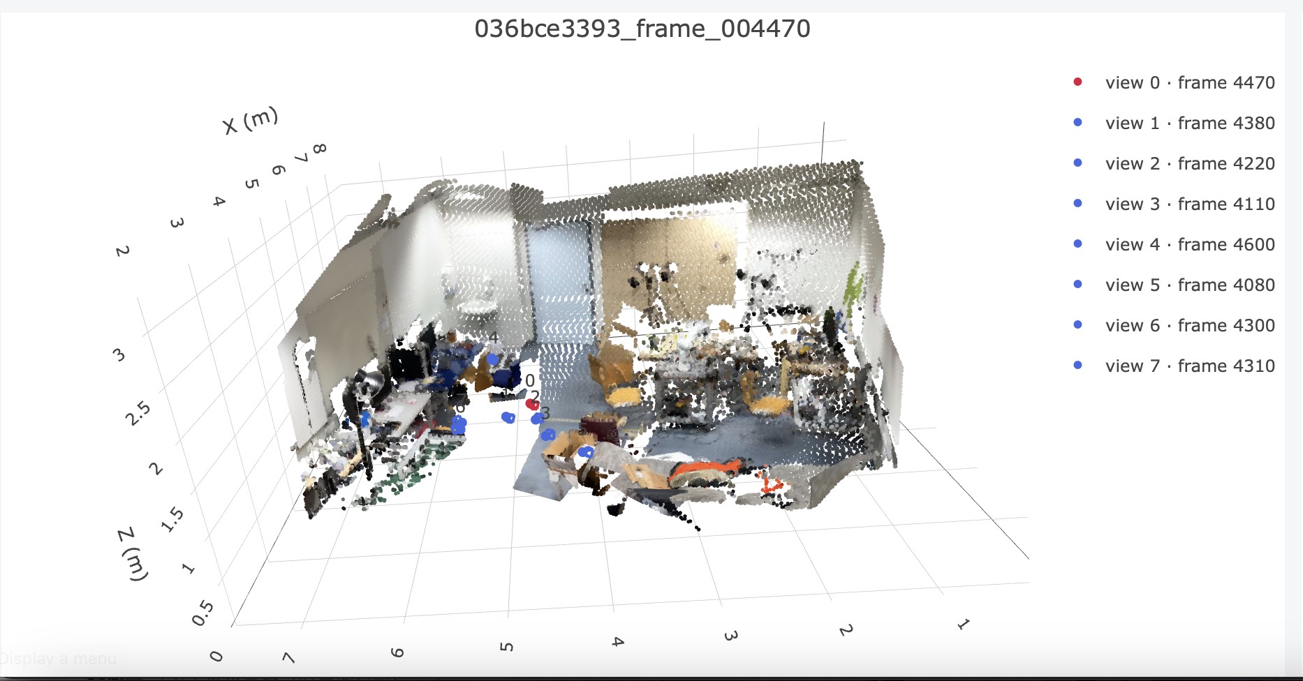
1.3. Camera and Depth Canonicalization
After Q1.3, visualize canonicalized geometry. Camera 0 should be identity, with the valid-point centroid approximately 1 unit from the origin:
python scripts/visualize_data.py --stage canonicalization --num-scenes 5 --max-points 10000 --output outputs/canonicalizationScreenshot
Note: I tried to put them together, but if I scroll down, the visualization will disappear so I made the screenshot separately. But all of them are correspondent to each other and of the same scene.
| Scene | Img | First camera center & centroid distance |
|---|---|---|
| 1 |  |  |
| 2 |  | 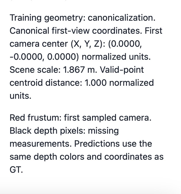 |
1.7. Final Check
python scripts/check_data.py --config configs/scannetpp/iphone/data.json --split train --max-samples 4check_data.py output
{ "split": "train", "dataset_samples": 224, "checked_samples": 4, "samples": [ { "sequence_name": "e050c15a8d_frame_007080", "views": 8, "resolution": 224, "valid_depth_fraction": 0.9779127240180969, "max_reprojection_error_px": 0.00010810750973178074, "max_ray_reprojection_error_px": 9.448717901250347e-05, "centroid_distance": 1.0 }, { "sequence_name": "5f99900f09_frame_002820", "views": 8, "resolution": 224, "valid_depth_fraction": 0.9903116226196289, "max_reprojection_error_px": 0.00011108566104667261, "max_ray_reprojection_error_px": 0.00011108566104667261, "centroid_distance": 0.9999999403953552 }, { "sequence_name": "47b37eb6f9_frame_002720", "views": 8, "resolution": 224, "valid_depth_fraction": 0.9609947800636292, "max_reprojection_error_px": 9.770392352947965e-05, "max_ray_reprojection_error_px": 8.897326188161969e-05, "centroid_distance": 1.0 }, { "sequence_name": "4c5c60fa76_frame_006690", "views": 8, "resolution": 224, "valid_depth_fraction": 0.7516716122627258, "max_reprojection_error_px": 0.00010193614434683695, "max_ray_reprojection_error_px": 9.423537994734943e-05, "centroid_distance": 0.9999999403953552 } ], "batch_shapes": { "rgb": [ 2, 8, 3, 224, 224 ], "depth": [ 2, 8, 1, 224, 224 ], "depth_valid": [ 2, 8, 1, 224, 224 ], "K": [ 2, 8, 3, 3 ], "frame_numbers": [ 2, 8 ], "T_world_from_camera": [ 2, 8, 4, 4 ], "original_world_from_reference": [ 2, 4, 4 ], "scene_scale": [ 2 ], "points_world": [ 2, 8, 3, 224, 224 ], "ray_origins": [ 2, 8, 3, 224, 224 ], "ray_directions": [ 2, 8, 3, 224, 224 ], "plucker": [ 2, 8, 6, 224, 224 ] }}Discussions
Canonicalization
Canonicalization is important, it changes different scenes into the same scale. We can look at the picture in 1.2, and compare with the in 1.3, the scale in 1.2 was from 0 to 8, but in 1.3 is within 2. This allows network in later implementation to learn without knowing about different scales, and makes it simpler than putting scale S into loss like the way in
World-space ray directions
This allows pixels to have information of directions. In the picture above, we can notice that there are triangles representing camera of different positions and their directions of ray. With this, we can recognise whether two rays has eye on the same point.
Plücker moment
The
2. Novel-View Synthesis with Mini-LVSM (40 points)
2.1. Overfitting (10 points)
Once your implementation is complete, check that it can memorize one fixed batch before full training:
python -m models.lvsm.train --overfit 2000 --output-dir outputs/lvsm_overfitCheck that the loss decreases and PSNR reaches about 30 dB or more, and inspect outputs/lvsm_overfit/val_epoch000.png.
Submission (Q2.1): Include the final overfit PSNR and the
val_epoch000.pngvisualization on your assignment webpage.
Overfit PSNR
PSNR: 34.09 dB
SSIM: 0.9156
Overfit visualization

2.2. Training and Evaluation (30 points)
python -m models.lvsm.train --config configs/lvsm.jsonThis prints train and validation metrics every epoch and saves best.pt, last.pt, log.jsonl and val_epoch*.png (visualizations) under outputs/lvsm/.
Evaluate best.pt with ablations over the number of source views and the target-ray conditioning.
python -m models.lvsm.eval --checkpoint outputs/lvsm/best.pt --num-source-views 1 2 4 --conditioning correct shuffled noneSettings:
correct uses the true target rays, shuffled uses the rays of a different target view, and none uses all-zero rays.
Metrics:
| Metric | Definition | Better |
|---|---|---|
| PSNR | How close the predicted image is to the real one, in dB, based on the pixel error (MSE) | Higher |
| SSIM | How similar the structure (edges, contrast, local patterns) of the two images is, from 0 to 1 | Higher |
Training curves
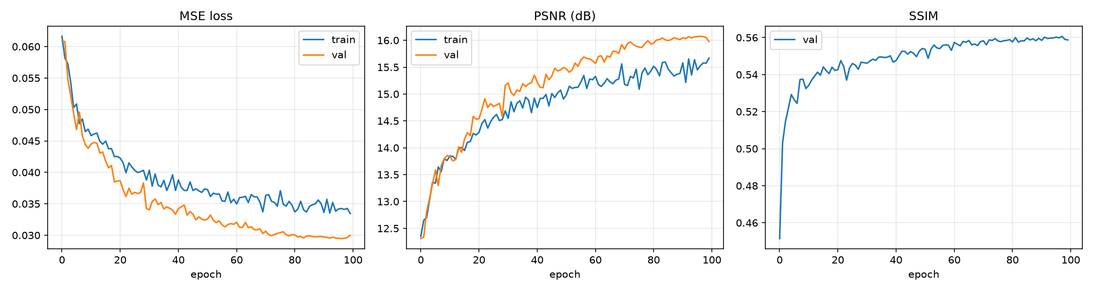
Results for ablation setting
| Source views (S) | Conditioning | PSNR (dB) | SSIM |
|---|---|---|---|
| 1 | correct | 15.14 | 0.5578 |
| 1 | shuffled | 11.83 | 0.4894 |
| 1 | none | 12.49 | 0.5270 |
| 2 | correct | 16.07 | 0.5598 |
| 2 | shuffled | 11.52 | 0.4751 |
| 2 | none | 12.45 | 0.5280 |
| 4 | correct | 16.76 | 0.5745 |
| 4 | shuffled | 11.65 | 0.4782 |
| 4 | none | 12.49 | 0.5410 |
Training visualizations
Epoch 0
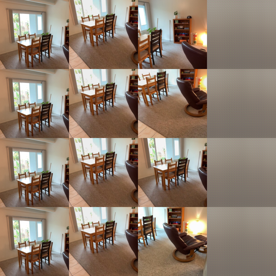
Epoch 50
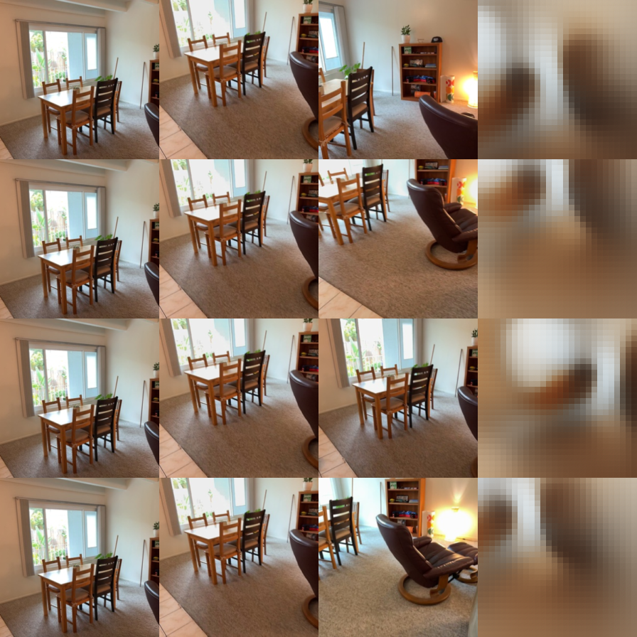
Epoch 95
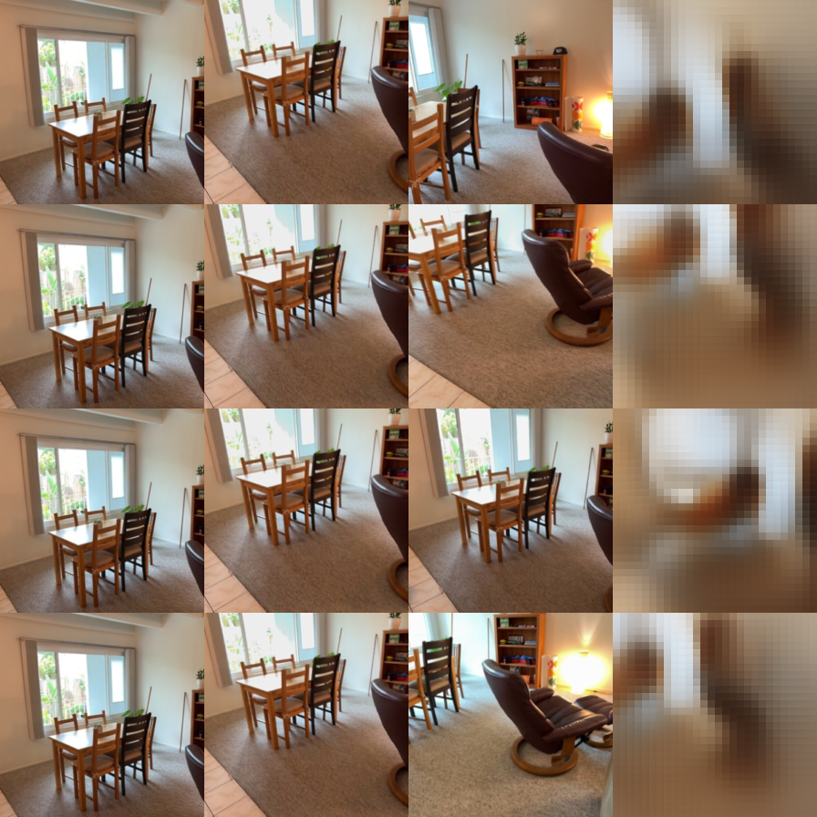
Evaluation visualizations
| Setting | Visualization |
|---|---|
| S=1, correct | 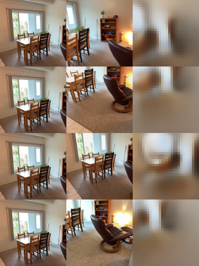 |
| S=1, shuffled | 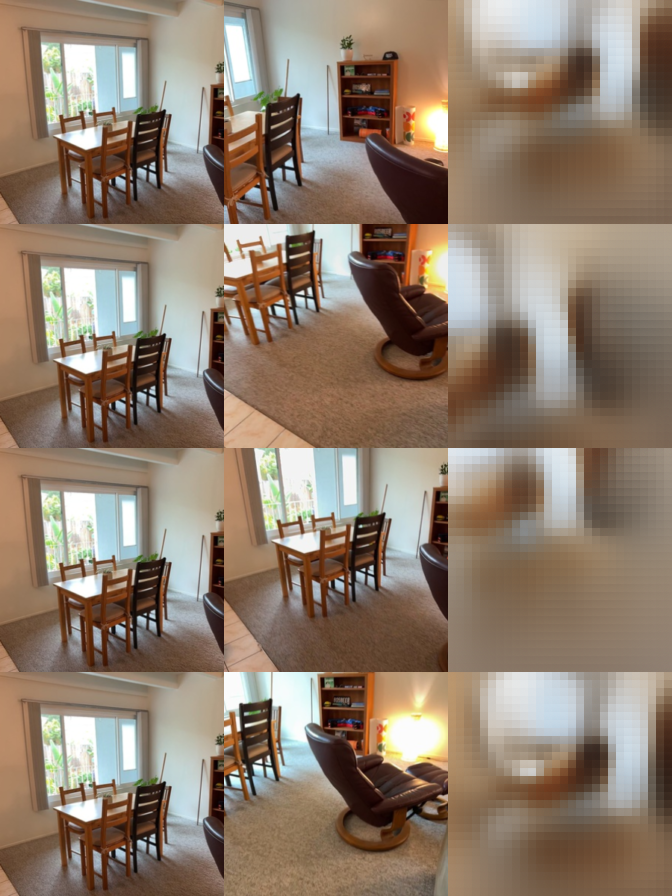 |
| S=1, none |  |
| S=2, correct | 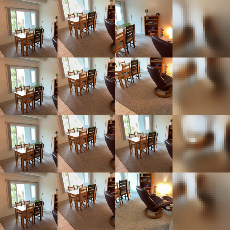 |
| S=2, shuffled | 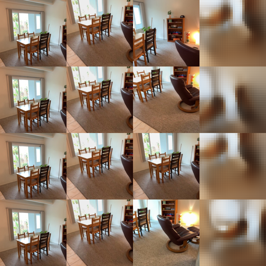 |
| S=2, none | 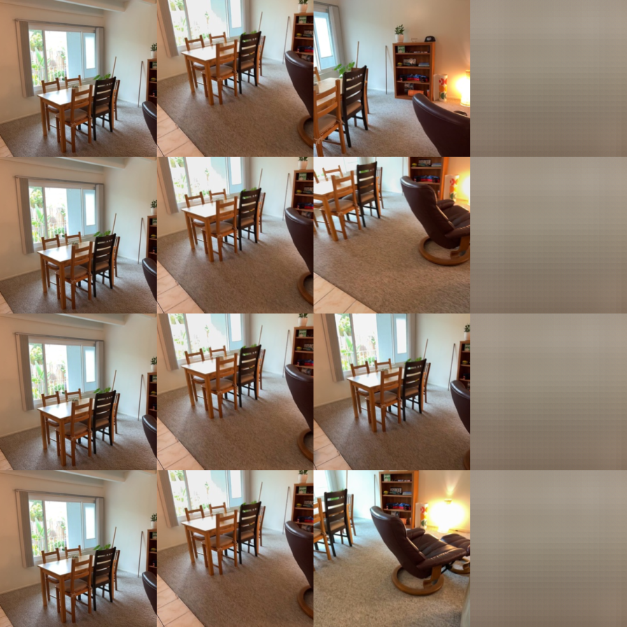 |
| S=4, correct | 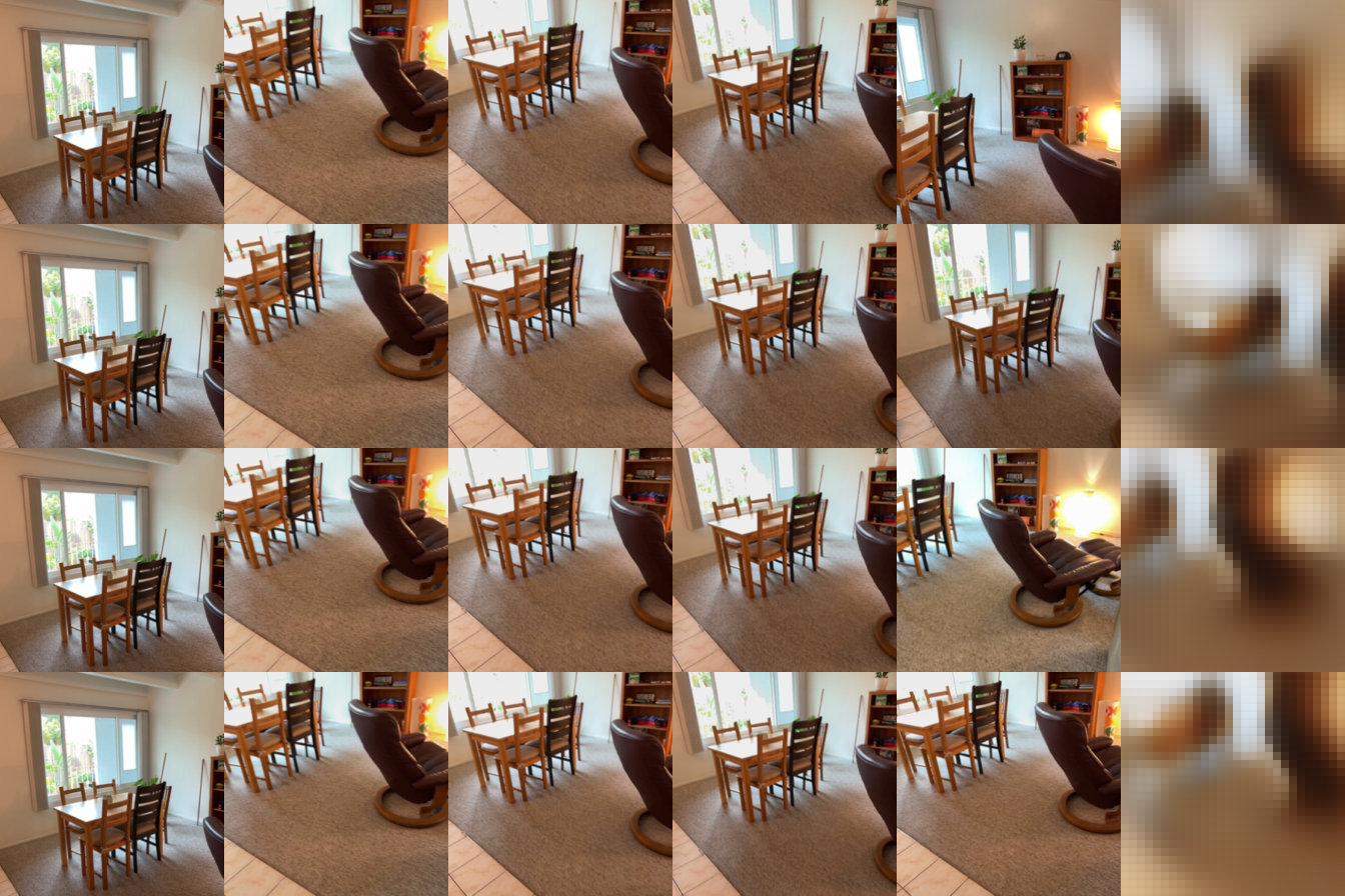 |
| S=4, shuffled | 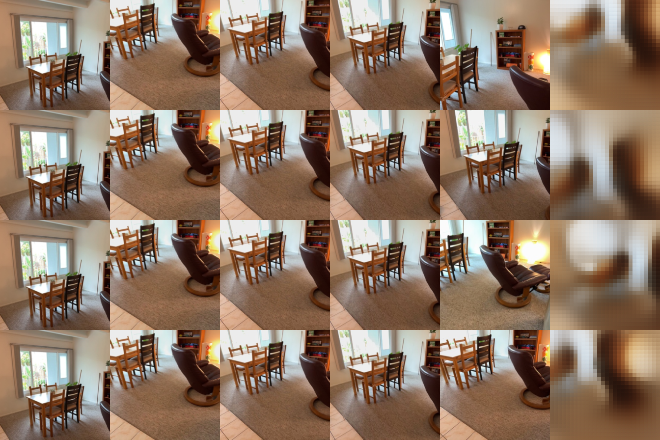 |
| S=4, none | 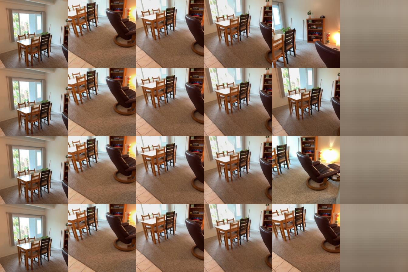 |
Training settings
Using almost default settings except changed batch size from 4 to 2.
Training took around 2h on a 8GB 3070Ti Laptop GPU. Setting batch size low to suit on 8GB RAM for GPU.
Discussions
The overall picture is vague, and I noticed in Piazza discussion that it is normal within this number of epochs and settings.
We can notice that the model act the best in the setting of S equals four and correct for the shuffled one the performance is worse. But it's interesting that shuffled has picutre that's funny and clearer than none, but it has worse PSNR (11.65) than none (12.49), it seems that giving a wrong perspective will ever make things worse(?) not really. It might also due to the bias of PSNR and SSIM score.
For the S=4, it's the clearest picture out of prediction, S=4 > S=2 > S=1. It is easy to understand because if we have more perspectives, then we have better understanding of a certain scene.
2.3. Bonus: Analysis and Exploration (10 points)
Training view count: Train with a different number of source views, or a random number per step. How does this change evaluation with 1, 2 and 4 source views?
Question & Experimental setting
Question: Train with a different number of source views, change numer of source views into 4, figure out what affect will be made on metrics and visualization.
Experimental setting: only change num_source_views from 2 to 4 in the config file, keep all others the same.
Result & Conclusion
| Eval S | Conditioning | Train S=2 PSNR | Train S=2 SSIM | Train S=4 PSNR | Train S=4 SSIM |
|---|---|---|---|---|---|
| 1 | correct | 15.14 | 0.5578 | 15.15 | 0.5574 |
| 1 | shuffled | 11.83 | 0.4894 | 11.86 | 0.4865 |
| 1 | none | 12.49 | 0.5270 | 12.35 | 0.5322 |
| 2 | correct | 16.07 | 0.5598 | 16.24 | 0.5595 |
| 2 | shuffled | 11.52 | 0.4751 | 11.50 | 0.4673 |
| 2 | none | 12.45 | 0.5280 | 12.32 | 0.5292 |
| 4 | correct | 16.76 | 0.5745 | 17.25 | 0.5766 |
| 4 | shuffled | 11.65 | 0.4782 | 11.47 | 0.4625 |
| 4 | none | 12.49 | 0.5410 | 12.37 | 0.5401 |
Visualization
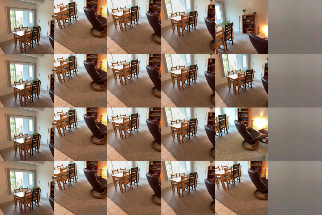
Epoch 0
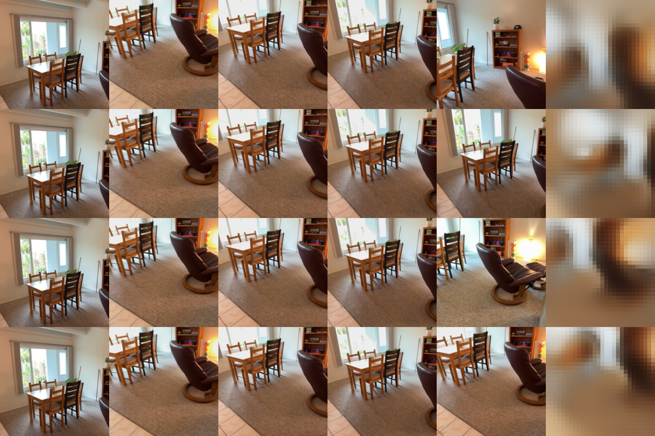
Epoch 50
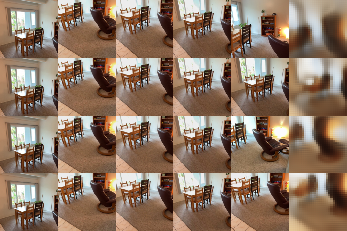
Epoch 95
Explanation & Limitation
We can notice both in metric results and visual results that when number of source views turn into 4, the performance is better with PNSR and SSIM: 17.25 and 0.5766, compared to 16.76 and 0.5745 in the last case. Because if we have more perspectives during training, the model is more used to 4 pictures and seems can get more information out of the same setting. But it is interesting that for S=1 during testing didn't change much, even drop some in SSIM.
Limitation: During training, with more numbers of source view, the training speed get slower.
3. Multi-View Geometry with Mini-VGGT (40 points)
3.1. Overfitting (10 points)
Default model: A frozen DINOv2 ViT-B/14 encoder feeds 8 frame/global transformer pairs (16 blocks; width 384; 6 attention heads). The camera head adds 4 cross-view transformer blocks, and the depth head decodes patch features with RGB refinement.
python -m models.vggt.train --config configs/vggt.json --overfit --output outputs/vggt_overfitInspect outputs/vggt_overfit/loss_curve.png and outputs/vggt_overfit/visualization/index.html. Check that loss decreases and predicted geometry approaches GT.
Submission (Q3.1): Include the overfit loss curve image (total, camera and depth loss) and screenshots comparing GT and predicted geometry on your assignment webpage.
Loss curve image

Screenshot
| GT geometry | Predicted geometry |
|---|---|
 |  |
3.2. Training and Evaluation (30 points)
Once single-scene overfitting works, train on the full training split. We recommend starting with the defaults in configs/vggt.json. You may adjust other hyperparameters while keeping num_views=8 and sampling_range=32.
xxxxxxxxxxpython -m models.vggt.train --config configs/vggt.json --output outputs/vggt_trainFor four GPUs, replace python with torchrun --standalone --nproc_per_node=4. The script saves loss_curve.png, last.pt, best.pt and visualization/index.html under the output directory. The HTML compares GT and predicted geometry on validation scenes; best.pt is selected by validation loss.
To continue an interrupted run with its saved settings, optimizer and schedule:
xxxxxxxxxxpython -m models.vggt.train --resume outputs/vggt_train/last.ptEvaluate best.pt on validation and test using 8 views from the first 32 prepared frames, 224px and seed 825. These flags override the checkpoint's data settings. Run the full splits without --max-batches:
xxxxxxxxxxpython -m models.vggt.eval --checkpoint outputs/vggt_train/best.pt --split val --eval-root data/scannetpp/prepared_eval --num-views 8 --eval-num-frames 32 --image-size 224 --seed 825 --report outputs/vggt_train/metrics.json --visualization outputs/vggt_train/visualization/index.htmlpython -m models.vggt.eval --checkpoint outputs/vggt_train/best.pt --split test --eval-root data/scannetpp/prepared_eval --num-views 8 --eval-num-frames 32 --image-size 224 --seed 825 --report outputs/vggt_train/test_metrics.jsonMetrics:
| Metric | Definition | Better |
|---|---|---|
| Depth AbsRel | Mean abs(pred − GT) / GT over valid pixels | Lower |
| Depth δ1 | Fraction with max(pred/GT, GT/pred) < 1.25 | Higher |
| Rotation AUC | Pairwise relative rotation accuracy | Higher |
| Translation AUC | Pairwise translation-direction accuracy, allowing sign ambiguity | Higher |
| Joint Pose AUC | Uses the larger rotation/translation error per pair | Higher |
Report each AUC at 5°, 15° and 30°; values range from 0 to 1. Depth metrics use all GT-valid pixels; translation/joint AUC excludes pairs with undefined GT translation direction.
Submission (Q3.2): Include the normal-training loss curve image (total, camera and depth loss), validation/test metrics, and screenshots comparing GT and predicted geometry for four different scenes. State your training settings and briefly discuss errors on held-out scenes.
Loss curve image

Validation/test metrics
| Metric | Val | Test |
|---|---|---|
| Depth Abs Rel | 0.1699 | 0.1718 |
| Depth delta1 | 0.7501 | 0.7634 |
| Rotation AUC 5° | 0.2054 | 0.2293 |
| Rotation AUC 15° | 0.5208 | 0.5688 |
| Rotation AUC 30° | 0.7019 | 0.7511 |
| Translation AUC 5° | 0.0128 | 0.0084 |
| Translation AUC 15° | 0.0834 | 0.0648 |
| Translation AUC 30° | 0.2050 | 0.1864 |
| Joint Pose AUC 5° | 0.0036 | 0.0043 |
| Joint Pose AUC 15° | 0.0583 | 0.0497 |
| Joint Pose AUC 30° | 0.1807 | 0.1712 |
Screenshot
I tried my best to adjust to the best position but still somewhat different:(
| Scene | GT geometry | Predicted geometry |
|---|---|---|
| 1 |  | 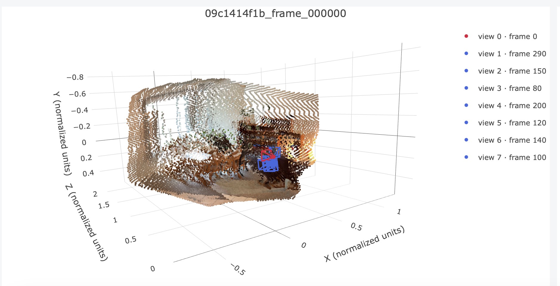 |
| 2 |  | 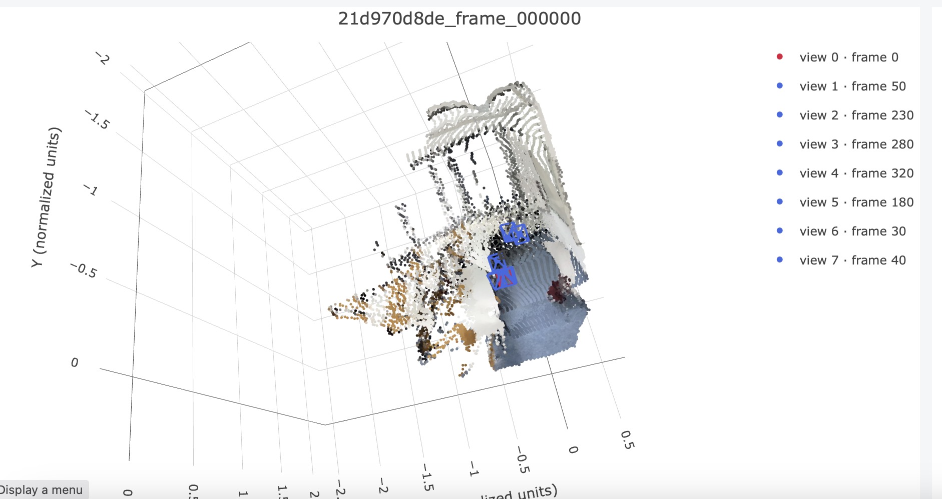 |
| 3 |  | 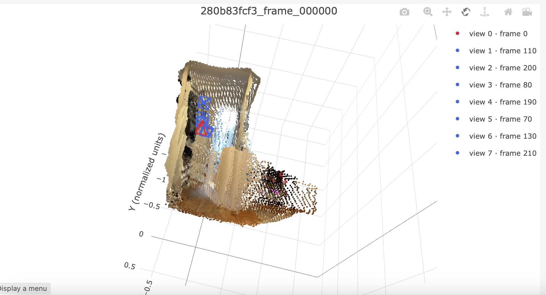 |
| 4 |  | 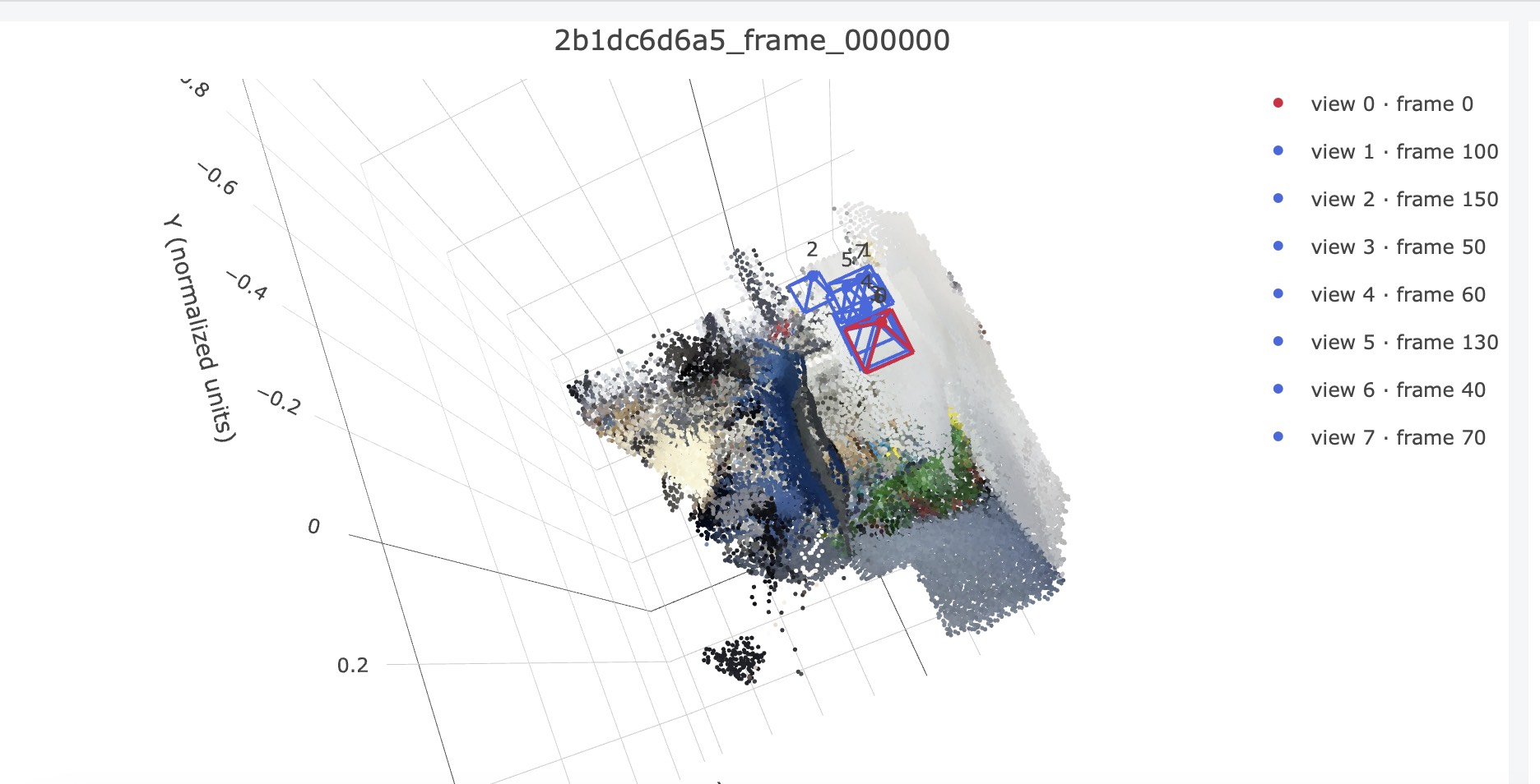 |
Training setting
Using almost default settings except changing batch size from 16 to 1, and changed number of workers from 8 to 2.
Training took around 12h on a 8GB 3070Ti Laptop GPU. Setting numbers above low to suit on the 8GB 3070Ti GPU, and limited RAM on WSL system.
Discussion
We can notice that in overfitting, on the Screenshot, the prediction is almost the same as the ground truth. This is because when training, the network optimize the network to just fit the data. It is like opening test answer to a student and the student will get full points, So we need held out, split the testing and training datasets.
On the test datasets, the network seems to predict vague on the edge of pictures. It is because on the edge of pictures, the information within the frame is less, covered by less viewpoints. And in the first case, the edges of desks and chairs aren't clear. But the depths and the relative position of objects is correct.