Volume Rendering, NeRF, and 3D Gaussian Splatting
Goals: In this assignment, you will set up a differentiable rendering pipeline and implement neural volume rendering techniques including NeRF, VolSDF, and 3D Gaussian Splatting.
Table of Contents
Volume Rendering, NeRF, and 3D Gaussian SplattingTable of Contents1. Differentiable Volume Rendering1.3. Ray sampling (5 points)Visualization1.4. Point sampling (5 points)Visualization1.5. Volume rendering (20 points)Visualization2. Optimizing a basic implicit volume2.1. Random ray sampling (5 points)2.2. Loss and training (5 points)2.3. Visualization3. Optimizing a Neural Radiance Field (NeRF)Visualization4. NeRF Extras4.1 View Dependence (10 points)Visualization5. 3D Gaussian Rasterization5.5 Perform Splatting6 Training 3D Gaussian Representations (15 points)6.2 Perform Forward Pass and Compute LossResultsGif7 Extensions7.1 Rendering Using Spherical Harmonics (10 points)Gif comparisonImage comparison
1. Differentiable Volume Rendering
1.3. Ray sampling (5 points)
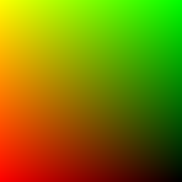
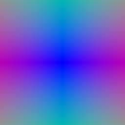
Take a look at the render_images function in volume_rendering_main.py. It loops through a set of cameras, generates rays for each pixel on a camera, and renders these rays using a Model instance.
Visualization
My own run results:
1.4. Point sampling (5 points)
Visualization
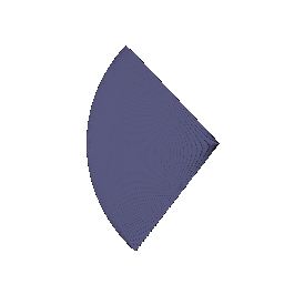
Use the render_points method in render_functions.py in order to visualize the point samples from the first camera.
My own run results:
1.5. Volume rendering (20 points)
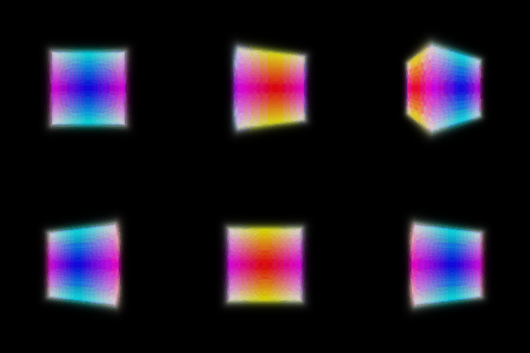
Finally, we can implement volume rendering! With the configs/box.yaml configuration, we provide you with an SDFVolume instance describing a box. You can check out the code for this function in implicit.py, which converts a signed distance function into a volume. If you want, you can even implement your own SDFVolume classes by creating new signed distance function class, and adding it to sdf_dict in implicit.py. Take a look at this great web page for formulas for some simple/complex SDFs.
Visualization
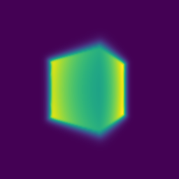
By default, your results will be written out to images/part_1.gif. Provide a visualization of the depth in your write-up. Note that the depth should be normalized by its maximum value.
My own run results:
2. Optimizing a basic implicit volume
2.1. Random ray sampling (5 points)
Since you have now implemented a differentiable volume renderer, we can use it to optimize the parameters of a volume! We have provided a basic training loop in the train method in volume_rendering_main.py.
Depending on how many sample points we take for each ray, volume rendering can consume a lot of memory on the GPU (especially during the backward pass of gradient descent). Because of this, it usually makes sense to sample a subset of rays from a full image for each training iteration. In order to do this, implement the get_random_pixels_from_image method in ray_utils.py, invoked here:
xxxxxxxxxxxy_grid = get_random_pixels_from_image(cfg.training.batch_size, image_size, camera) # TODO: implement in ray_utils.py2.2. Loss and training (5 points)
| Value (Rounded) | |
|---|---|
| Box center | (0.25, 0.25, -0.00) |
| Box side lengths | (2.01, 1.50, 1.50) |
2.3. Visualization
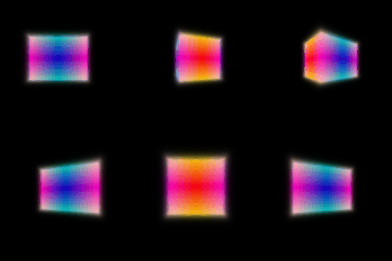
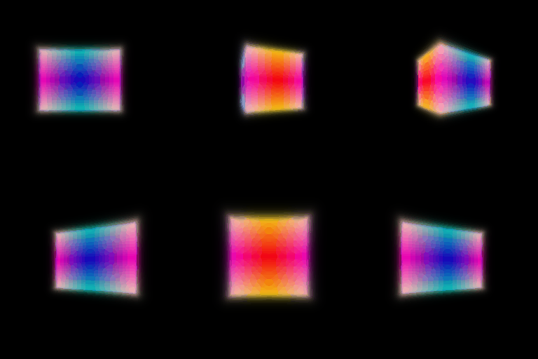
The code renders a spiral sequence of the optimized volume in images/part_2.gif.
Mine:
TA's:
3. Optimizing a Neural Radiance Field (NeRF)
Visualization
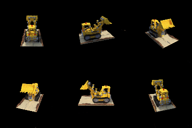
You can train a NeRF on the lego bulldozer dataset with
xxxxxxxxxxpython volume_rendering_main.py --config-name=nerf_legoThis will create a NeRF with the NeuralRadianceField class in implicit.py, and use it as the implicit_fn in VolumeRenderer. It will also train a NeRF for 250 epochs on 128x128 images.
Result:
4. NeRF Extras
4.1 View Dependence (10 points)
Add view dependence to your NeRF model! Specifically, make it so that emission can vary with viewing direction. You can read NeRF or other papers for how to do this effectively --- if you're not careful, your network may overfit to the training images. Discuss the trade-offs between increased view dependence and generalization quality.
Visualization
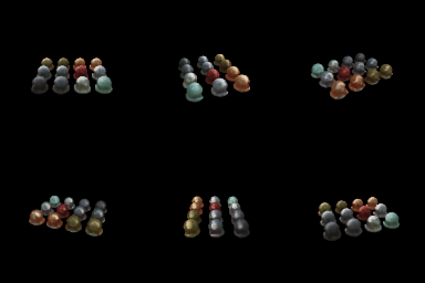
Explanation: with direction, the matrial of the balls are clearer, more likely to be metals. In different angles, the reflection, the highlight are different. But the real color of the ball looks to be unchanged, more similar to real world scenario. How to avoid overfitting: If rely on direction too much, the color can be also wrong. So we need to prevent over fitting. Only add direction after the network, before the color, avoid adding it into density. And avoid putting too much network layers around direction.
5. 3D Gaussian Rasterization
In this section, we will implement a 3D Gaussian rasterization pipeline in PyTorch. The official implementation uses custom CUDA code and several optimizations to make the rendering very fast. For simplicity, our implementation avoids many of the tricks and optimizations used by the official implementation and hence would be much slower. Additionally, instead of using all the spherical harmonic coefficients to model view dependent effects, we will only use the view independent compoenents.
5.5 Perform Splatting
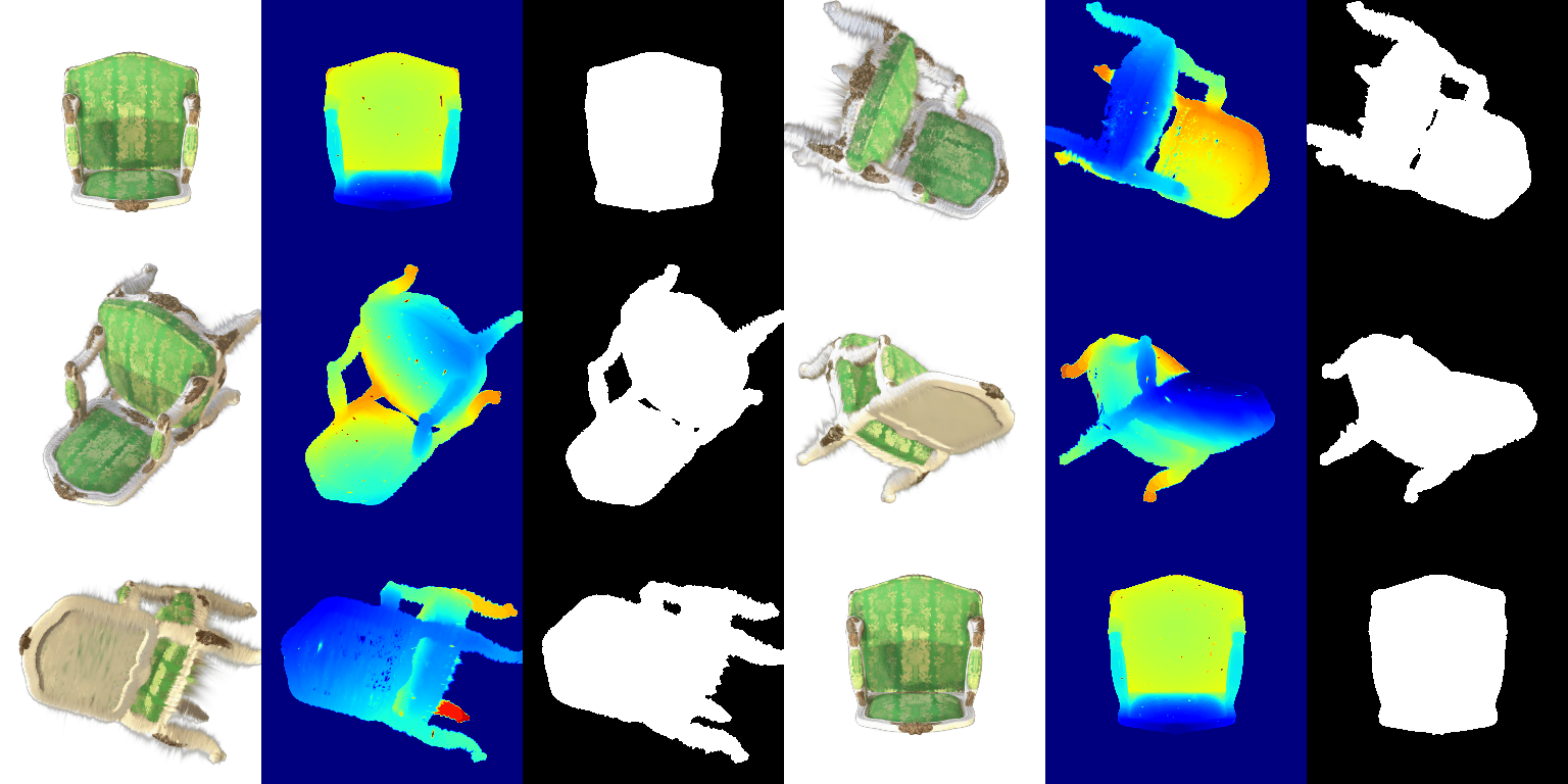
Test the rendering code by running python render.py. The output is as listed:
6 Training 3D Gaussian Representations (15 points)
6.2 Perform Forward Pass and Compute Loss
Results
Number of iterations: 1000
| No. run | means | scales | colours | opacities | PSNR | SSIM |
|---|---|---|---|---|---|---|
| 1 | 0.01 | 0.01 | 0.01 | 0.01 | 28.822 | 0.933 |
| 2 | 0.001 | 0.01 | 0.01 | 0.01 | 29.508 | 0.941 |
| 3 | 0.0002 | 0.01 | 0.05 | 0.05 | 28.737 | 0.930 |
| 4 | 0.0001 | 0.01 | 0.01 | 0.01 | 28.904 | 0.932 |
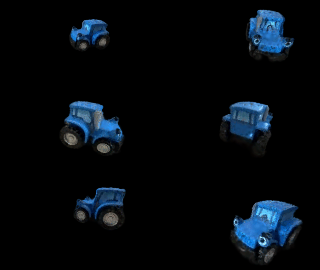
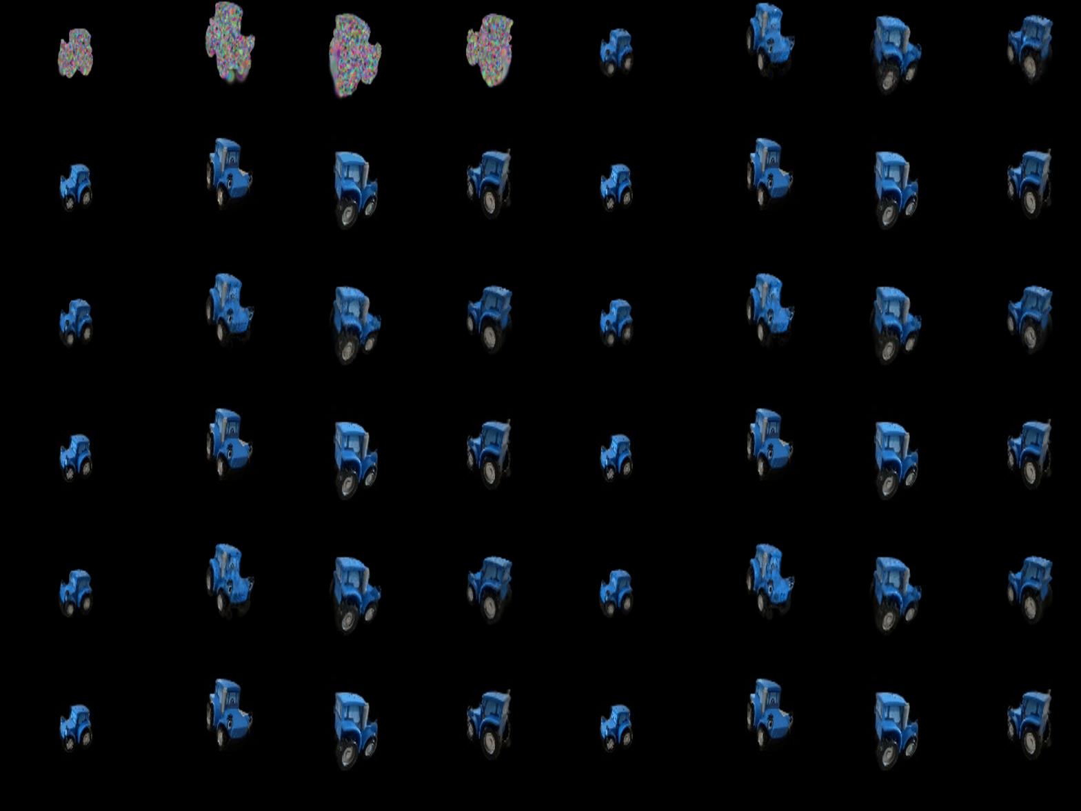
To test the learning rates, I conducted more than 5 groups of running and took the most representative 4 results and put them here, we can notice that run 2 with a not big nor small learning rate for means has better results.
Because means is the most important factor in gaussian, the position of gaussian decides the shape of the render result. So I mainly changed learning rate of means to test the results.
When the learning rate of mean is too small, the result converges slowly in limited iterations. When the learning rate of mean is too big, the result is less presice.
Gif
7 Extensions
7.1 Rendering Using Spherical Harmonics (10 points)
In this section, we will explore rendering 3D Gaussians with associated spherical harmonic components. We will add support for spherical harmonics such that we can run inference on 3D Gaussians that are already pre-trained using the original repository (we will not focus on training spherical harmonic coefficients).
Gif comparison
Gif in 7.1, with spherical harmonic:
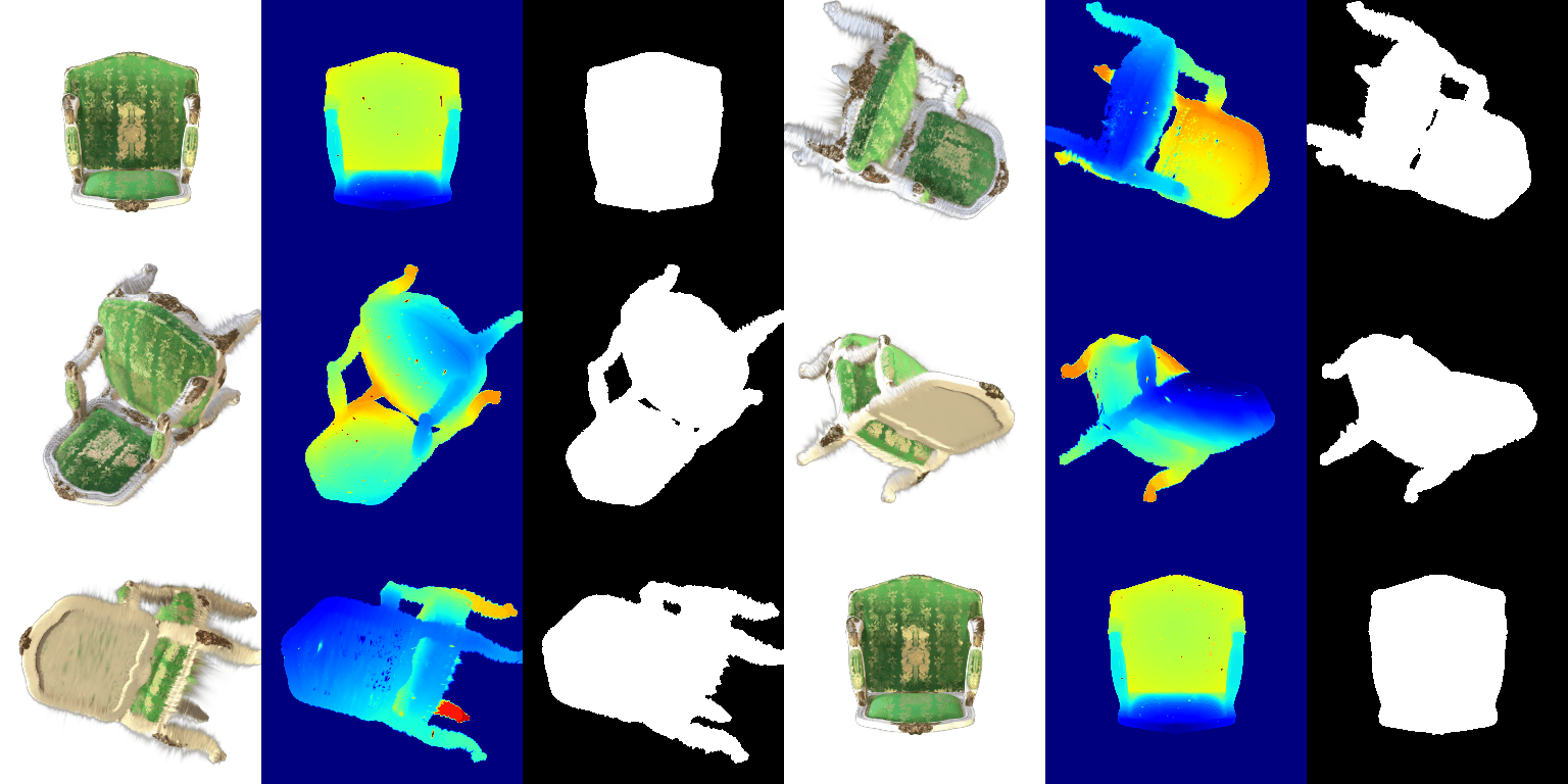
Gif in 5.5, without spherical harmonic:
Explanation: looking at the gif, the overall color of 7.1 is darker than 5.5, and shapes are similar, and the reflection in 7.1 looks more real. The gold pattern is more explicit in 7.1 rendering. The depth and mask are the same.
Image comparison
| Frame | 5.5 | 7.1 | Explanation |
|---|---|---|---|
| 3 | 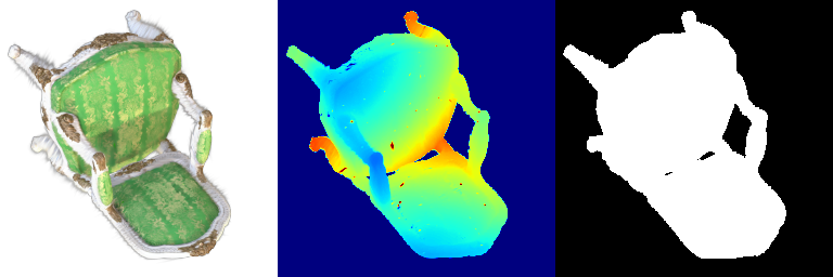 | 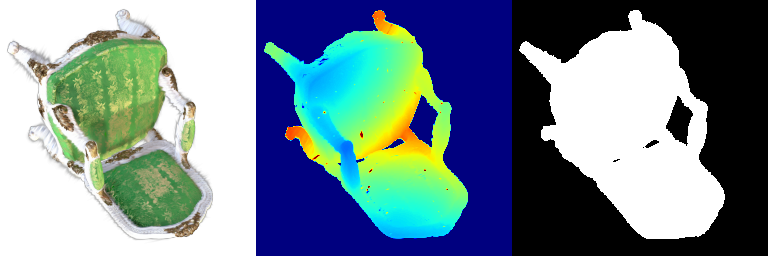 | 7.1 has daker chair color, and more explicit gold pattern. |
| 15 | 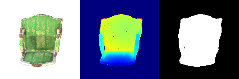 | 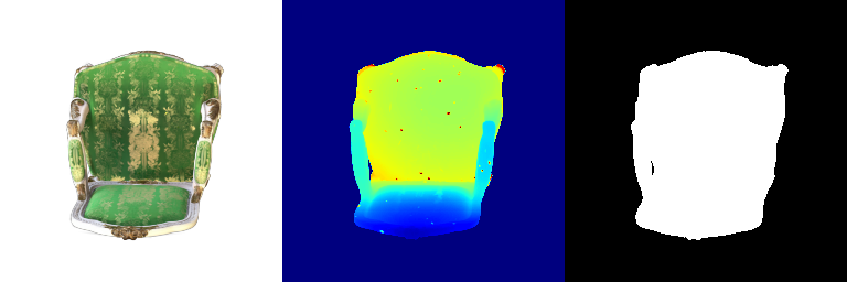 | 7.1 has more explict chair frame. the color is more vivid. The shades area is darker. |
| 27 | 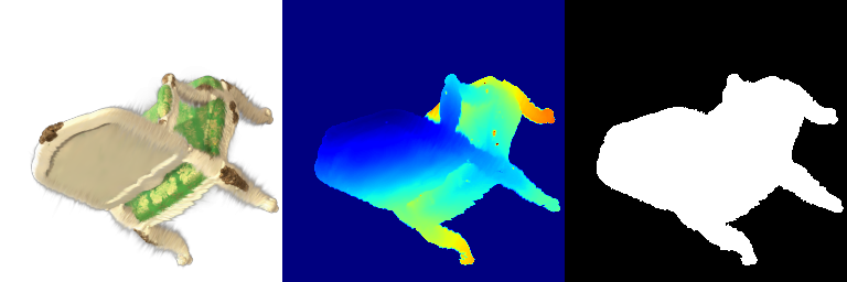 | 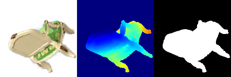 | almost similar, as the back of the chair has no shades and reflections. In the corner, 7.1 rendering has clearer shades. |