
Andrew ID: robertre
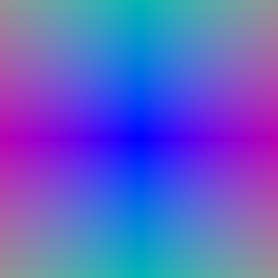
Left: xy grid. Right: ray directions.
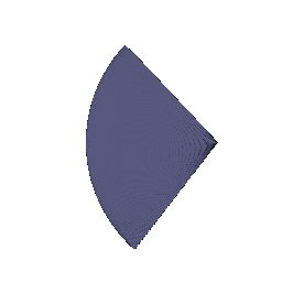

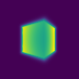
Left: spiral rendering. Right: depth map, normalized by its maximum.
| x | y | z | |
|---|---|---|---|
| Box center | 0.25 | 0.25 | 0.00 |
| Box side lengths | 2.01 | 1.50 | 1.50 |


There exists a tradeoff between view-dependence and generalization. A model with view dependence allows the color of a point to change as the viewing angle changes, which is good for capturing reflections and other challenging details. If view dependence doesn't exist in a network, then the color would be an average taken from all the different viewing angles. However, by adding view dependence to the model, the model could focus on getting per view effects right while slightly worsening the underlying geometry to make the training views look good, which could hurt the novel views. In this case, I make the density independent of the viewing angle because density is the underlying geometry, while making the colors change based on the views.

Left: one network, 128 samples per ray. Right: coarse network with 64 samples, then fine network with the 64 coarse + 128 new samples.
Compared to the one-pass network, which only does 128 evaluations per ray, the coarse + fine network requires 64 evaluations for the coarse pass and 64+128=192 evaluations for the second pass, which totals to 256 evaluations. In practice, I measured ~65 it/s for the one-pass network and ~29 it/s for the coarse + fine network, with more memory usage as well. However, the coarse + fine network allows us to better recover fine details by allocating evaluation points more intelligently thanks to the initial coarse stage. However, the gain in quality is a bit difficult to tell at 128x128 resolution.


alpha controls the density / opacity when inside an object. The larger the alpha, the faster the ray stops once it crosses the surface. beta controls how confident we are about the surfaces. The higher the beta, the larger the variance is, meaning we are less certain about the true location of the surface.
I used: alpha = 10, beta = 0.05, eikonal weight = 0.02. The model is trained for 250 epochs with a learning rate of 5e-4. I also used geometric initialization (from: https://arxiv.org/abs/1911.10414), so the SDF starts as a sphere of radius 1. With the default initialization, the SDF became negative everywhere and the surface collapsed. The eikonal weight keeps the network close to a valid SDF, and beta = 0.05 is small enough to give a sharp surface.
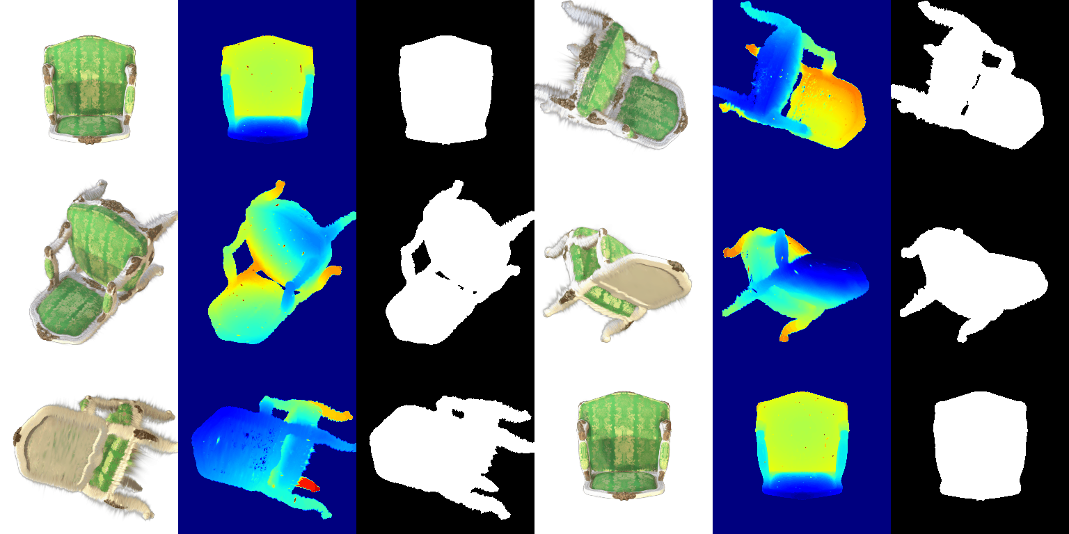
| Parameter | Learning rate |
|---|---|
| Opacities | 0.05 |
| Scales | 0.005 |
| Colours | 0.005 |
| Means | 0.0005 |
Iterations: 1000. PSNR: 29.85. SSIM: 0.944.
Training progress:

Final renders:

Without spherical harmonics (5.5):
With spherical harmonics:
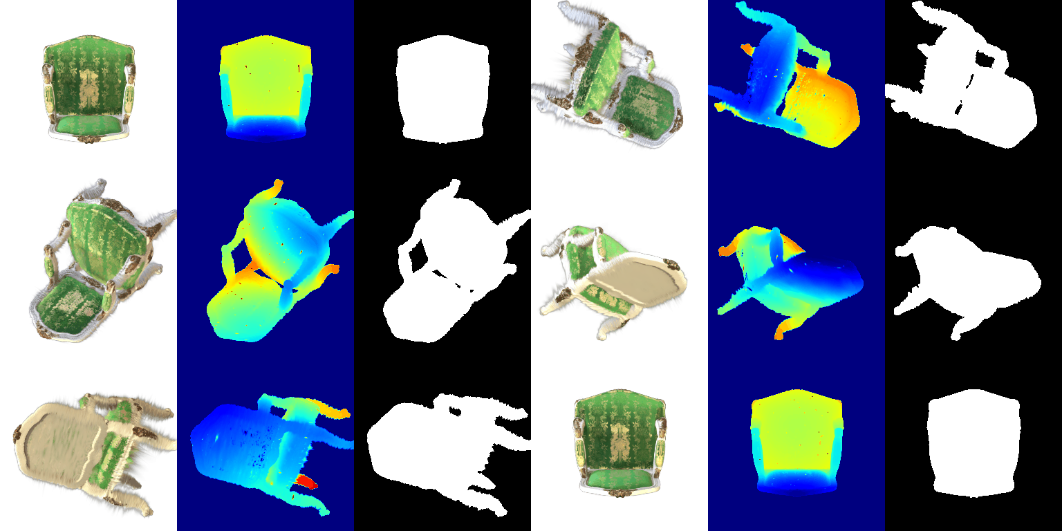
Same view, without (left) and with (right) spherical harmonics:

With spherical harmonics, the fabric is darker and the gold pattern stands out more.

With spherical harmonics, the back cushion has a bright gold highlight in the middle and darker sides.

With spherical harmonics, the shadow is less abrupt on the cushion of the chair.
Without spherical harmonics, each Gaussian has one color averaged over all views. With spherical harmonics, the color changes with the view, which adds shading and highlights on the shiny fabric and gold trim.
| Method | PSNR | SSIM |
|---|---|---|
| Baseline (6.2 setup, random init) | 18.46 | 0.678 |
| Improved | 21.52 | 0.752 |
| Parameter | Baseline learning rate | Improved learning rate |
|---|---|---|
| Opacities | 0.05 | 0.05 |
| Scales | 0.005 | 0.005 |
| Colours | 0.005 | 0.005 |
| Means | 0.0005 | 0.005 |
| Rotations (quaternions) | not trained (isotropic) | 0.001 |
Iterations: 1000 for both runs. In the improved run, an exponential schedule multiplies all learning rates by 0.1 over the 1000 iterations.
Baseline training progress:
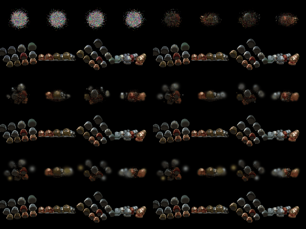
Improved training progress:
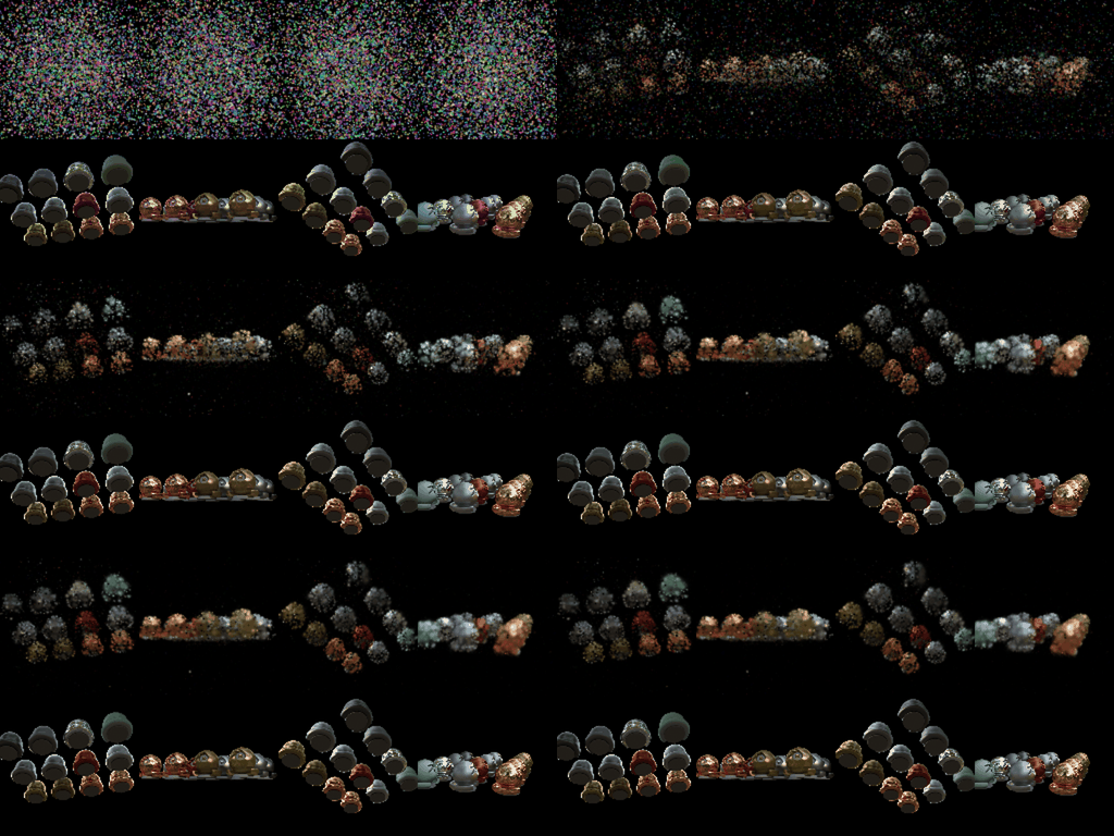
Improved final renders:

With the improved model, the PSNR improved to 21.52 and the SSIM improved to 0.752. I have made three improvements to the training. First, I made the initialization range wider. This is based on the observation from the training progression for the baseline, where Gaussians have to be moved from the center of the scene to cover more objects on the edges. The wider initialization makes the coverage wider to cover more objects earlier in the training. I also increased the learning rate with an exponential decay schedule for the means of the Gaussians so that they can move more freely to model all the different objects in the scene. I also made the Gaussians anisotropic so that they can stretch in each of the 3 dimensions. The 3 improvements allowed the model to capture all objects and higher fidelity for each object.