
psalmon
All experiments ran on one NVIDIA T4 (16 GB). Part A has every section, including two NeRF extensions (4.1 view dependence and 4.3 VolSDF). Part B has every section, including both extensions (7.1 and 7.2).
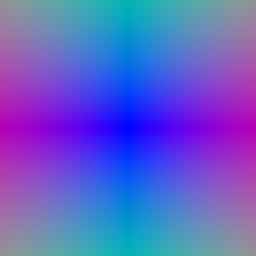
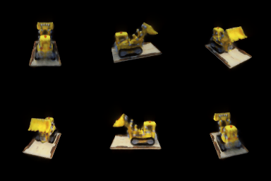
get_pixels_from_image builds a W by H grid of pixel centers mapped linearly to [-1, 1]. get_rays_from_pixels appends depth 1 to each NDC point, lifts it into the world with camera.unproject_points, and starts every ray at the camera center, pointing (unit length) through its lifted pixel.
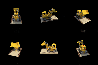
Pixel grid (left, vis_grid) and absolute ray directions (right, vis_rays) for the first camera.
StratifiedRaysampler uses n_pts_per_ray equally spaced depths from min_depth to max_depth and returns origin + t * direction for each. During training only, each depth is jittered uniformly within its bin, so over many steps the network is queried continuously along the ray. Rendering is deterministic.
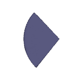
render_points).For each sample, alpha = 1 - exp(-sigma * delta), transmittance T is torch.cumprod of 1 - alpha shifted by one sample (so T = 1 for the first sample), and the weight is T * alpha. Summing these weights against per-sample color gives the pixel color; summing them against sample distance gives depth.
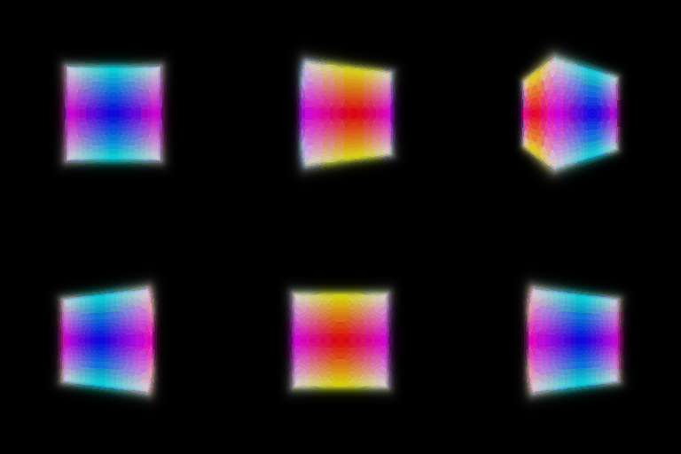

Spiral rendering of the box (left) and depth for the third camera, normalized by its maximum (right).
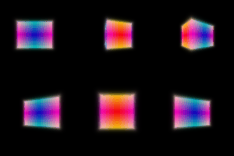
get_random_pixels_from_image shuffles the pixel grid with torch.randperm and returns batch_size of them, so no pixel repeats within a batch. Training minimizes squared color error on those pixels. After 1,000 epochs:
| x | y | z | |
|---|---|---|---|
| Box center | 0.25 | 0.25 | 0.00 |
| Box side lengths | 2.01 | 1.50 | 1.51 |
NeuralRadianceField encodes position with 6 harmonic frequencies. A 6-layer, 128-unit ReLU MLP processes the encoding, and the encoding is concatenated back in before layer 3. Density comes from a single linear unit passed through ReLU. Another linear layer feeds a 64-unit head with a sigmoid that gives color. The loss is MSE on 1,024 random rays per step, with 128 stratified samples per ray. I used nerf_lego.yaml unchanged: 250 epochs at 128 by 128, learning rate 5e-4 decaying by 0.8 every 50 epochs.
Held out PSNR over the 100 validation views is 24.34 dB (train views: 24.57 dB).
With use_view_dirs: True, the color head also receives the viewing direction, encoded with 2 harmonic frequencies. The encoding joins only after the density head has branched off, so density stays a function of position alone and only color can change with viewpoint. This follows the original NeRF design. Both materials models use nerf_materials.yaml (learning rate 1e-4, 250 epochs).
| Materials, 128 by 128 | Train PSNR | Validation PSNR |
|---|---|---|
| Position only | 23.46 dB | 23.35 dB |
| With view dependence | 24.16 dB | 24.01 dB |
PSNR is averaged over the 100 train and 100 validation views, using the epoch 200 checkpoints.
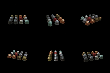
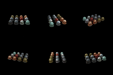
Left: position only. Right: with view dependence.
What changes. In the position-only model, every 3D point must commit to a single color, so a highlight that a sphere shows from some training cameras is blended into its surface color for every view. The glossy and metallic spheres come out with dull, spread-out highlights. With the direction as input, the same spheres have brighter, more compact highlights, which a viewpoint-dependent color can represent and a fixed color cannot. The held-out views improve by 0.66 dB.
Generalization. The danger of a direction input is that it gives the network a second way to reduce training error. A pixel it gets wrong because the geometry is wrong can instead be patched by a color that only appears from that training camera. That is NeRF++'s shape-radiance ambiguity: the training views are fit, but novel views expose the wrong shape. How much room the network has for this depends on how much freedom the direction gets. In my model the direction cannot reach the density at all, it is concatenated only into the final 64-unit color layer, and its encoding uses just 2 frequencies (sin and cos of each direction component at frequencies 1 and 2). That last choice is a low-pass limit: color can change gradually over a sphere's highlight, but not flip between neighboring training cameras. The measured gap between train and validation PSNR is small for both models (0.11 dB position-only, 0.15 dB with direction), so on this scene the extra freedom bought accuracy rather than memorization. Raising the direction frequencies, or feeding the direction into the trunk, would buy more training fit at the risk of that gap widening.

nerf_materials_highres.yaml settings with view dependence, rendered at epoch 200). The sphere materials and their highlights are clearer than at 128 by 128. With 128 samples per ray and a 128-unit MLP, fine texture inside the spheres stays slightly soft.Network. NeuralSurface encodes position with 6 harmonic frequencies. A 6-layer, 128-unit MLP with Softplus (beta = 100) activations follows. Softplus keeps the SDF smooth and its gradient well defined, whereas ReLU would make it piecewise linear. The last layer outputs the signed distance plus a 128-dimensional geometry feature. A 2-layer color MLP maps that feature and the positional encoding to RGB through a sigmoid. The network uses geometric initialization (as in SAL/IDR): the weights are set so that the SDF starts as a sphere of radius 1, with the positional-encoding inputs initially zeroed. Training therefore begins from a valid, closed surface instead of an arbitrary function.
Losses. The eikonal loss is mean((|grad d| - 1)^2) over random points in the bounding box, at weight 0.02, added to the color MSE.
SDF to density. Following VolSDF, sigma(x) = alpha * Psi_beta(-d(x)), with Psi_beta the Laplace CDF of scale beta. The two parameters play separate roles. alpha sets how opaque the material is: it is the ceiling the density approaches inside the object, so it controls how quickly a ray is stopped once it has entered. beta sets how sharp the boundary is, measured in scene units. Concretely, with signed distance d (positive outside):
d | -3 beta | -beta | 0 | +beta | +3 beta |
|---|---|---|---|---|---|
sigma / alpha | 0.98 | 0.82 | 0.50 | 0.18 | 0.02 |
So almost all of the transition happens within about 3 beta of the zero level set. With the default beta = 0.05 that band is roughly 0.3 units thick, about a tenth of the bulldozer's size. Shrinking beta toward 0 turns the density into a hard on/off occupancy.
Results. All runs use volsdf_surface.yaml (alpha = 10, eikonal weight 0.02, 250 epochs at 128 by 128) and change only beta. PSNR is averaged over the 100 validation views.
| beta | Validation PSNR | Surface |
|---|---|---|
| 0.01 | 22.39 dB | Sharpest. The base plate is a thin sheet with ragged edges. |
| 0.05 (default) | 22.22 dB | Clean, but the base plate is a rounded, bulging slab. |
| 0.2 | 21.24 dB | Blobby. The base is a thick, rounded slab, and the thin arm is lost, so the bucket floats detached. |
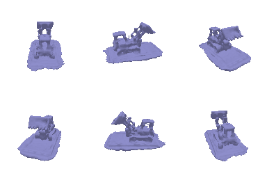
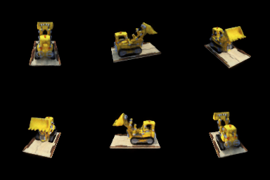
Default settings (beta = 0.05): surface extracted with marching cubes at SDF = 0 (left) and volume rendering (right).
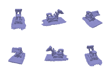
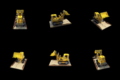
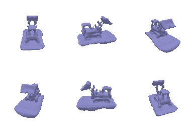
beta = 0.01 (left pair) and beta = 0.2 (right pair): geometry, then color.
Q1: bias from high vs low beta. The sweep above shows it directly. At beta = 0.2 the transition band is about 1.2 units thick, wider than the bulldozer's arm. Any structure thinner than the band cannot produce a crisp edge in the render, so the photometric loss has no reason to keep it, and the optimization trades it for a smooth, rounded shape that renders a similar soft image: the arm vanishes and the base swells into a slab. High beta therefore biases the SDF toward over-smoothed, rounded geometry that loses thin parts. At beta = 0.01 the band is only about 0.06 units, so the render changes sharply exactly where d crosses zero, and the loss pins the zero level set to the image edges. The bias goes the other way: toward thin, sharp surfaces, at the cost of ragged edges where few rays constrain the shape, like the rim of the base plate.
Q2: which trains more easily. High beta. Training starts from a sphere that is in the wrong place. To move that surface, a ray needs samples where sigma has a useful slope with respect to d, and that only happens inside the transition band. A wide band means a large fraction of the 128 samples on every ray fall in it from the first iteration, so the surface receives a strong, smooth signal even when it is far from the target. A narrow band is hit by only a few samples per ray (with 128 samples over 4 units, spacing is about 0.03, comparable to the whole band at beta = 0.01), so the gradient is sparse and depends on exactly where the samples land.
Q3: which gives the more accurate surface. Low beta, as long as it converges. With a thin band, the depth at which a ray becomes opaque coincides with the zero crossing of d, so the extracted mesh is the surface the images actually see. With a thick band, opacity accumulates well before d = 0, so the images can be matched by a level set that is offset or smoothed, and the mesh inherits that error. Validation PSNR follows the same order in my runs: 21.24 dB at 0.2, 22.22 dB at 0.05, and 22.39 dB at 0.01.
Chosen settings. I report beta = 0.05 as the main result even though 0.01 scores 0.17 dB higher, because its mesh is cleaner: the arm and bucket stay attached, and the base has none of the fraying seen at 0.01. I left alpha = 10 unchanged. With a sample spacing of about 0.03, one sample deep inside the object has opacity 1 - exp(-10 · 0.03), about 26%, so a ray is mostly stopped within a few samples of entering and the color comes from near the surface rather than from inside it. The eikonal term (weight 0.02) is applied at random points throughout the bounding box, so d stays a true distance away from the surface too, which keeps marching cubes at d = 0 well defined.
Implementation summary:
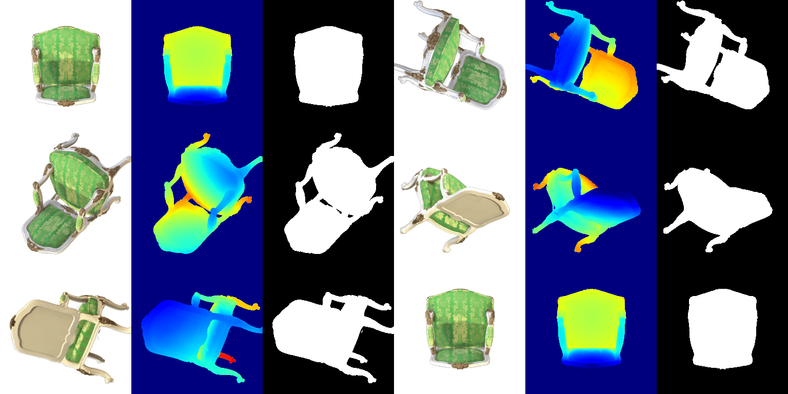
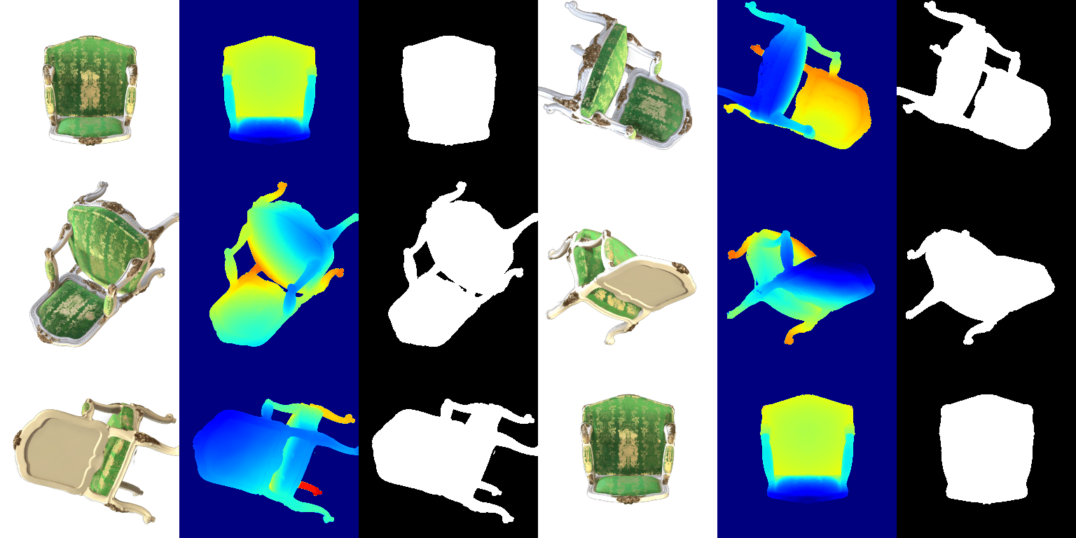
R S ST RT from the quaternion and scales. In the isotropic case this reduces to s2 I, so the quaternion is never used.J W Σ WT JT, where J comes from _compute_jacobian.transform_points_screen.-½ dT Σ-1 d per Gaussian and pixel.torch.cumprod over the depth-sorted 1 - alpha, starting from the transmittance left over by the previous mini-batch.Σ wi ci, Σ wi zi, and Σ wi, with w = alpha T.Which W? My compute_cov_2D passes unit tests 1 and 3 but not 2 and 4, which check the anisotropic 2D covariance and expect W = camera.R. I used W = camera.RT on purpose. _compute_jacobian differentiates the projection with respect to view-space coordinates, so W must map world-space offsets into view space. PyTorch3D stores R for right-multiplication of row vectors (Xview = Xworld R + T), so for the column-vector product J W Σ WT JT that map is RT. The pre-trained chair is a direct test. It has 284k anisotropic Gaussians, and with W = R the elongated ones along the frame and legs are drawn in the wrong orientation, so the edges grow streaks. With RT they line up with the surfaces. The instructor's Piazza answer allows W = R; I kept RT for every result, and swapping that single line makes all four tests pass. For isotropic Gaussians the choice cannot matter, since rotating s2 I by any W returns s2 I, so question 6 and the 7.2 baseline are unaffected.
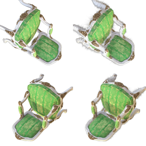
W = RT (used). Right column: W = R (matches unit tests 2 and 4). Two views.Speed. The renderer evaluates every Gaussian at every pixel. Writing the 2 by 2 quadratic form out in closed form, rather than as a batched einsum, and compositing color and depth with a matrix product made rendering 3.2 times faster. A 256 by 256 frame of the 284k-Gaussian chair then takes about 36 seconds on the T4.
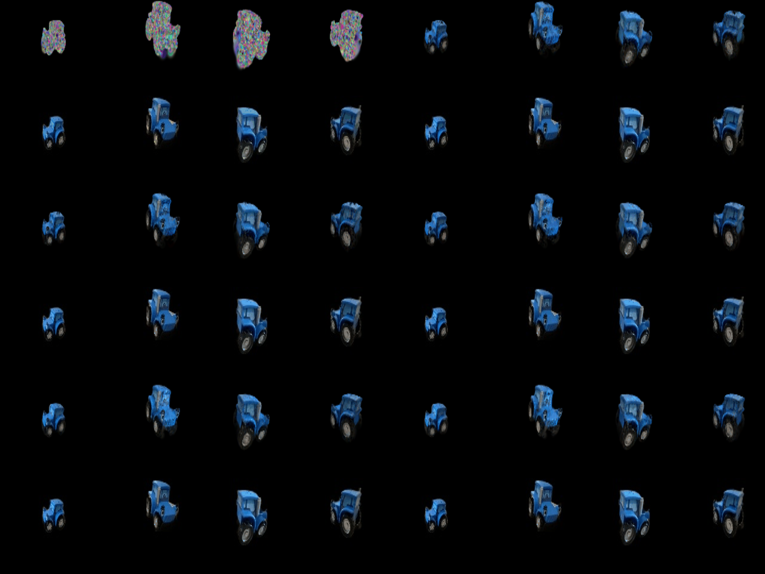
make_trainable turns on gradients for means, pre_act_scales, colours, and pre_act_opacities. The quaternions stay frozen, because an isotropic covariance s2 I does not depend on them (check_if_trainable rejects them in this mode). Training renders one random training view per iteration against a black background and minimizes the L1 photometric error with Adam, one parameter group per tensor:
| Tensor | Adam learning rate | Reasoning |
|---|---|---|
means | 0.0005 | The 10k-point cloud already lies on the truck (extent about 5 units), so positions only need small corrections. |
pre_act_scales (log space) | 0.005 | A step of 0.005 in log scale changes a radius by 0.5%, which is gentle enough not to blur neighbors. |
colours | 0.02 | Random initial colors need to reach the right RGB within a few hundred steps. |
pre_act_opacities (logit) | 0.05 | They start at logit 8 (opacity 0.9997); a large step lets unneeded Gaussians fade out. |
After 1,000 iterations, the held-out test views give PSNR 29.53 and SSIM 0.940.

The ply file stores 48 numbers per Gaussian: an RGB triple for each of the 16 real spherical harmonic basis functions of degree 0 to 3. colours_from_spherical_harmonics reshapes them to (N, 16, 3), evaluates the 16 basis polynomials at each Gaussian's unit viewing direction (from the camera center through the Gaussian's mean, computed in calculate_gaussian_directions), and takes the weighted sum. The final colour gets the same +0.5 offset and lower clip at zero that the DC colours received in question 5, so the two modes differ only by the view-dependent terms. The --use_sh flag of render.py selects the mode.
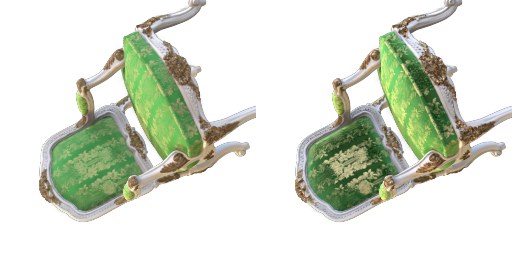
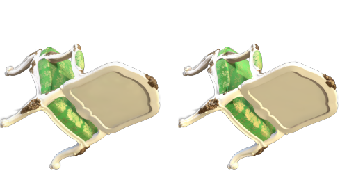
Left: DC term only (question 5.5). Right: all spherical harmonic coefficients (question 7.1).
In each comparison below, the DC-only render is on the left and the full SH render on the right, for the same frame.

The materials scene trains at 128 by 128 from 10,000 randomly initialized Gaussians and is evaluated on the 100 validation views.
| Iterations | PSNR | SSIM | |
|---|---|---|---|
| Baseline (Q6 recipe) | 1,000 | 18.54 | 0.679 |
| Improved | 4,000 | 24.71 | 0.899 |
Baseline. I reran train.py's recipe unchanged (isotropic, L1, question 6 learning rates, 1,000 iterations) on init_type="random". Its final renders show a hazy cluster of colored blobs in the middle of the frame, with the outer objects faint or missing. A quick look at the geometry explains why. The materials cameras sit 4.03 units from the origin with focal length 3.125 (NDC), so the visible region at the origin has a radius of about 4.03 / 3.125, roughly 1.3 units. The starter's random means come from N(0, 0.22), so about 99% of them start within 0.7 units of the origin. Adam moves a parameter by at most roughly its learning rate per step, so with a means rate of 0.0005 a Gaussian can travel at most about 0.5 units in 1,000 steps. The baseline cannot reach most of the scene in principle.
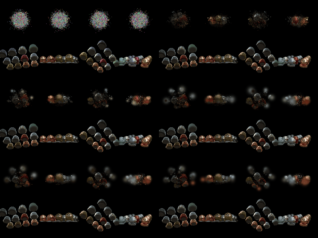
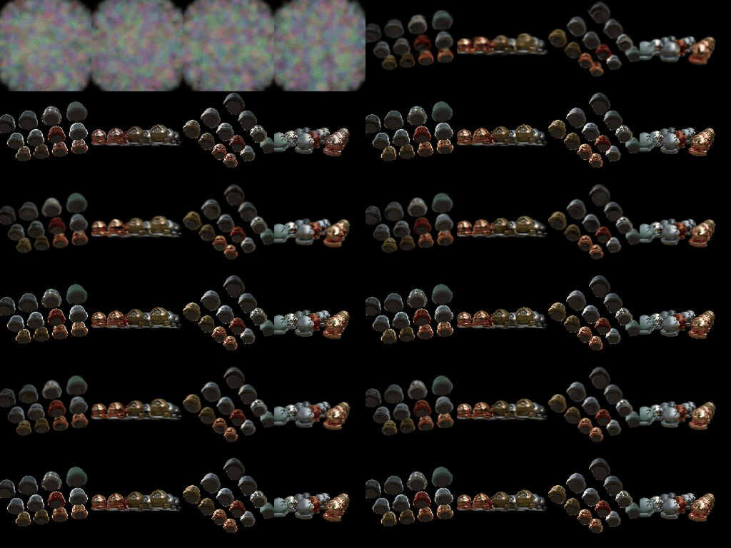
Training progress, baseline (left, every 20 iterations) and improved (right, every 100 iterations). In each, predictions are on top and ground truth on the bottom. Both GIFs are shown at half resolution.

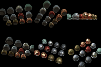
Final renders of the training views: baseline (left) and improved (right).
Improved recipe (train_harder_scene.py --mode improved). Each change targets a specific way the baseline falls short. The Gaussian count stays at 10,000, and everything starts from random positions, as required.
| Problem in the baseline | Change | Setting |
|---|---|---|
| Means start in a cluster the optimizer cannot escape (above). | Draw the random means uniformly from a ball that encloses the visible region, and size each Gaussian to that density. | Ball radius 1.5; initial radius = half the average spacing of 10k points in that ball. |
| Even after spreading out, the means still need to travel early on, but a large rate makes them jitter at the end. | Exponential decay of the means learning rate. | 0.0016 decaying to 1.6e-5 over training. |
| Starting nearly opaque (0.9997), the front-most random Gaussians hide everything behind them, so those get almost no gradient. | Start semi-transparent. | Initial opacity 0.12 (logit -2). |
| Round blobs cannot follow curved sphere surfaces or sharp silhouettes. | Anisotropic Gaussians with trainable rotation. | Quaternion learning rate 0.001. |
| Most of each image is black background, so L1 is small even when edges and patterns are blurred. | Mix in a structural term, as in the 3DGS paper. | Loss = 0.8 L1 + 0.2 (1 - SSIM), Gaussian window 11, sigma 1.5. |
| Random init wastes many Gaussians in empty space, where they fade to zero opacity and stop contributing. | Periodically move faded Gaussians onto useful ones (relocation in the style of 3DGS-MCMC; total count fixed). | Every 100 iterations, for the first 70% of training. |
| 1,000 iterations is too short for random initialization. | Train longer. | 4,000 iterations. |
Relocation details. A Gaussian counts as faded when its opacity is below 0.005. Each faded Gaussian picks a target among the remaining ones with probability proportional to opacity and copies its scale, rotation, and colour. It is placed at the target's mean plus Gaussian noise of the target's size. The target's opacity o is then shared: both copies get 1 - sqrt(1 - o), so the pair stacked together still blocks the same fraction of light (1 - (1 - o') 2 = o). The moved Gaussian's Adam statistics are zeroed. Over the run, the first round (iteration 100) found nothing to move, the count rose to a peak of 323 at iteration 600, and then dropped to roughly 110 to 130 per round by the last relocation.
Fitting it on the T4. Training splats in chunks of 5,000 Gaussians wrapped in gradient checkpointing, so only one chunk's per-pixel intermediates are kept at a time and are recomputed during the backward pass. This changes memory, not the result.
Discussion. Coverage of the scene appears to be the key fix. The improved model's progress GIF already shows all the spheres, blurred, at iteration 100, while the baseline never shows them in 1,000 iterations. I did not run a per-change ablation, so I cannot split the 6.2 dB gain among the individual changes. The main errors left are fine patterns inside some spheres and the sharp reflections on the metallic ones, since each Gaussian has a single view-independent colour.