Assignment 3: Volume Rendering, NeRF, and 3D Gaussian Splatting
Author: Po-Ting Ko
Andrew ID: potingk
A. Neural Volume Rendering
1. Differentiable Volume Rendering
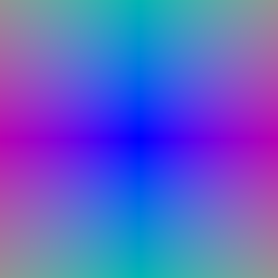
1.3 Ray sampling
Pixels are mapped to NDC [−1, 1] and unprojected with camera.unproject_points(..., from_ndc=True); rays start at the camera center.
| xy grid | Rays |
|---|---|
 |
 |
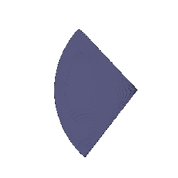
1.4 Point sampling
Uniform depths in [near, far], jittered within each bin during training. Samples of the first camera (every 16th ray):
1.5 Volume rendering
| Color | Depth (normalized by its maximum) |
|---|---|
 |
 |
2. Optimizing a basic implicit volume
Random rays: a random permutation of all pixels, keeping the first n_pixels. Loss: MSE on colors.
| Center | Side lengths | |
|---|---|---|
| Box | (0.25, 0.25, 0.00) | (2.01, 1.50, 1.51) |

The result matches the TA reference.
3. Optimizing a Neural Radiance Field (NeRF)
- Model: positional encoding (6 frequencies) → 6-layer MLP, width 128, ReLU, skip connection at layer 3 → density (ReLU) and color (Sigmoid).
- Training: the default
nerf_lego.yaml(250 epochs, 128 × 128, 1024 rays per step, 128 samples per ray); final loss 0.0039, about 17 min.

4. NeRF Extras
All Part 4 runs use TF32. Test PSNR is the mean over the 200 test views.
4.1 View Dependence
- Model: the density depends only on position. The color head also takes the harmonic embedding of the ray direction (2 frequencies), concatenated late, into the last small layer.
- Results: materials at 400 × 400 (
nerf_materials_highres_view.yaml); test PSNR 23.87.

Ground truth (left) and prediction (right) on test views:

Trade-off between view dependence and generalization (128 × 128)
| Model | Train PSNR | Test PSNR | Train − test |
|---|---|---|---|
| A: no view dependence | 23.46 | 23.09 | 0.37 |
| B: direction, 2 frequencies | 24.29 | 23.66 | 0.63 |
| C: direction, 8 frequencies | 24.39 | 23.71 | 0.68 |

- Gain. View dependence adds about 0.6 dB: the metal and copper spheres get highlights instead of a flat average color.
- Cost. The train/test gap grows with more view dependence (0.37 → 0.68 dB). A color that can change freely with the view can explain each training image with wrong geometry (the shape–radiance ambiguity), which causes overfitting at novel views.
- My design. Keeping density view-independent and using a few low frequencies only in the last layer keeps the effect smooth.
4.2 Coarse/Fine Sampling
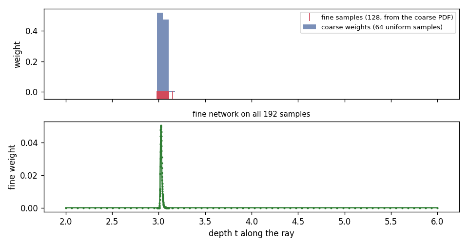
- Coarse pass. 64 stratified samples are rendered with a coarse network.
- Fine samples. Its weights form a PDF along the ray, and 128 more samples are drawn from it by inverse transform sampling.
- Fine pass. A second network renders all 192 samples.
- Loss. MSE(coarse) + MSE(fine).
On one ray, all 128 fine samples land within [2.98, 3.15] around the surface:
| Model | Queries per ray | Test PSNR | Train time | Render time per image |
|---|---|---|---|---|
| Single network, 128 samples (Part 3) | 128 | 24.21 | 11.7 min | 145 ms |
| Single network, 192 samples | 192 | 24.51 | 15.3 min | 212 ms |
| Coarse (64) + fine (64 + 128) | 256 | 24.43 | 19.6 min | 286 ms |
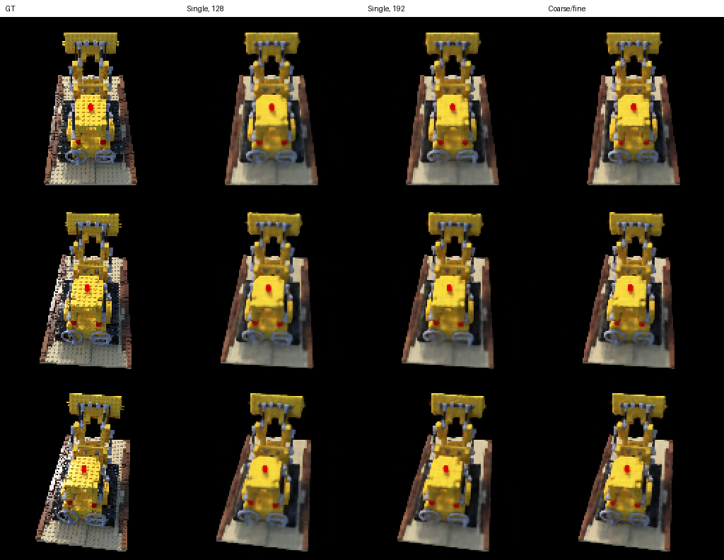
| Single, 128 | Single, 192 | Coarse/fine |
|---|---|---|
 |
 |
 |
- Speed. Coarse/fine is the slowest: training is 1.7× and rendering 2× slower than the single 128-sample network.
- Quality. It is +0.2 dB over 128 samples but not better than a single network with 192 samples. At 128 × 128 with a [2, 6] range, uniform samples are already dense enough. Importance sampling pays off at higher resolution, for larger scenes, or with fewer samples per ray.
4.3 VolSDF
- Distance MLP.
- 6 layers, width 128, with Softplus (β = 100).
- No output activation, since the SDF can be negative.
- Geometric (sphere) initialization.
- Color MLP. Two layers on the shared features, ending in a Sigmoid.
- Eikonal loss. mean(‖∇d‖ − 1)².
- SDF to density.
- α is the density inside the object: σ = α inside, 0 outside, α / 2 on the surface. A larger α makes the object opaque faster (within about 1 / α).
- β controls how sharp the surface is. Density rises from 0 to α over a band of width about β. As β → 0 the density becomes a step function at the surface.
Results
Lego, 250 epochs, α = 10, β = 0.05 (best); test PSNR 22.29:
| Geometry | Color |
|---|---|
 |
 |
Effect of β (rows: β = 0.01, 0.05, 0.2):

| β | Test PSNR | Zero level set − rendered depth | Weight outside the surface |
|---|---|---|---|
| 0.01 | 22.24 | −0.098 | 7% |
| 0.05 | 22.29 | −0.063 | 25% |
| 0.2 | 21.04 | +0.070 | 49% |
1. How does high β bias the learned SDF? What about low β? With a high β, half of the color comes from points outside the object. The network compensates by moving the zero level set inwards (+0.07 behind the rendered depth), giving a shrunken, smoothed surface where parts merge. With a low β, the density is concentrated at d = 0, so the SDF is nearly unbiased but sharp. The remaining offset comes from α, not β.
2. Would an SDF be easier to train with volume rendering and low β or high β? Why? High β. The gradient only flows through samples within a few β of the surface, so with a high β every ray gets a signal even when the surface is far from the object. Without geometric initialization, β = 0.2 still trains (21.39), but β = 0.01 fails (13.18):

3. Would you be more likely to learn an accurate surface with high β or low β? Why? Low β. The rendered color then comes from d = 0 itself, so the photometric loss constrains the surface directly, as the 7% weight outside the surface and the sharper mesh show. This works once training succeeds, for example with geometric initialization.
Settings. - β = 0.05 and α = 10 give the best PSNR with a clean surface. - Geometric initialization is what makes β ≤ 0.05 trainable. - Softplus keeps the SDF gradient smooth for the eikonal loss.
B. 3D Gaussian Splatting
5. 3D Gaussian Rasterization
- 5.1 Projection.
- Σ = R S Sᵀ Rᵀ.
- Σ' = J W Σ Wᵀ Jᵀ.
- 2D means come from
transform_points_screen. - 5.2 Evaluation. The quadratic form is expanded elementwise, 5.8× faster than
einsum. - 5.3 Filter and sort. Gaussians with view-space z < 0 are removed, and the rest sorted by z.
- 5.4 Alphas and transmittance. α = o · exp(power), and T is a
cumprod. - The provided
splatpassedtransmittance[-1]to the next mini-batch, missing the last Gaussian's (1 − α). I fixed this, so mini-batched and full rendering now match to 2e-7. - 5.5 Splatting. Color, depth and mask are Σ αT · (c, z, 1).
All 4 unit tests pass.

Note on W. The code uses W = R, as the unit tests and the course staff recommend. However, PyTorch3D uses row vectors (Xview = X R + T), so the true world-to-view rotation is Rᵀ. I checked this with Monte Carlo sampling: the covariance of projected samples matches W = Rᵀ, not W = R. The two agree for frontal views, but from oblique views W = R smears flat Gaussians. This does not affect isotropic Gaussians (Part 6).

6. Training 3D Gaussian Representations
- Setup.
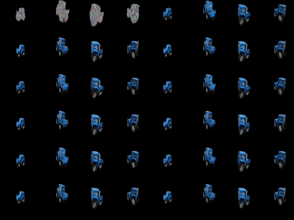
- 10,000 isotropic Gaussians initialized from the truck point cloud.
- L1 loss, Adam.
- 1000 iterations.
--gaussians_per_splat 2048.- Memory. Gradient checkpointing per mini-batch fits training in 8 GB: 3.3 GB at 0.66 s per iteration.
| Parameter | Learning rate |
|---|---|
| opacities (pre-sigmoid) | 0.05 |
| colours | 0.02 |
| scales (log) | 0.005 |
| means | 0.0005 |
| Iterations | Mean PSNR | Mean SSIM |
|---|---|---|
| 1000 | 29.70 | 0.943 |

7. Extensions
7.1 Rendering Using Spherical Harmonics
- Direction. For each Gaussian, d = normalize(μ − camera center).
- Colour. color = max(0, Σk ck Yk(d) + 0.5), with all 16 SH basis functions (degree 0–3), vectorized over the Gaussians.
- Check. My render differs from the reference frame by only 0.42/255 per pixel.
| Q5.5: DC only | Q7.1: full SH |
|---|---|
|
 |

- (a) Front view. With SH, the fabric is a darker, more saturated green, and the pattern and gold carvings are sharper. The DC-only render is washed out, about 20/255 too bright, because DC is the colour averaged over all directions.
- (b) Top-side view. With SH, the cushion is darker and the backrest shows stronger light and dark stripes. Without SH, all surfaces have nearly the same brightness.
- (c) Underside view. The two renders are almost identical (5/255): the matte beige bottom looks the same from every direction.
7.2 Training on a Harder Scene
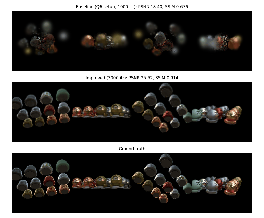
Materials scene, 128 × 128, random initialization. The baseline is the exact Q6 setup (isotropic Gaussians, Q6 learning rates, L1 loss, 1000 iterations).
| Method | Iterations | #Gaussians | Mean PSNR | Mean SSIM |
|---|---|---|---|---|
| Baseline (Q6 setup) | 1000 | 10,000 | 18.40 | 0.676 |
| Improved | 3000 | 8,216 | 25.62 | 0.914 |
Last frame of each progress GIF (baseline, improved, ground truth):
| Baseline training progress | Improved training progress |
|---|---|
 |
 |
| Baseline final renders | Improved final renders |
|---|---|
 |
 |
Modifications (compared to Q6):
- Initialization.
- Means are uniform in a ball of radius 1.3, which covers the scene; the default N(0, 0.2²) stays near the origin.
- Scales are set from the point spacing.
- Opacity starts at 0.1.
- Anisotropic Gaussians. Quaternions are trained (lr 0.001).
- Spherical-harmonic colours. Degree-3 coefficients are trained using the 7.1 code, with lr 0.01 for DC and 0.0005 for the higher orders.
- Loss. 0.8 · L1 + 0.2 · (1 − SSIM).
- Means learning rate. Exponential decay from 0.002 to 0.00002.
- Simplified density control. From iteration 200 to 2000, every 100 iterations:
- Densify the top 5% of Gaussians by positional gradient: clone the small ones and split the large ones (scale / 1.6).
- Prune Gaussians with opacity < 0.005.
- Training length. 3000 iterations.
Comparison. - Baseline. The Gaussians stay near the origin: at lr 0.0005 they can move only about 0.5. As a result, the outer spheres become large, blurry blobs. - Improved. The Gaussians find every sphere within a few hundred iterations. Pruning first removes Gaussians in empty space (10,000 → 5,426), then densification adds them back where detail is needed. - Caveat. There is no separate ablation per change.