Assignment 2: Single View to 3D
Author: Po-Ting Ko
Andrew ID: potingk
Note: all models in Q2 and Q3 were trained and evaluated with --load_feat (the provided precomputed ResNet-18 features).
1. Exploring loss functions
Each fit optimizes the shape directly (no network) to match one training chair from the R2N2 [1] / ShapeNet [2] data. Left: fitted source, right: target.
1.1 Fitting a voxel grid
Loss: binary cross-entropy on logits, F.binary_cross_entropy_with_logits(voxel_src, voxel_tgt).

1.2 Fitting a point cloud
Loss: chamfer distance, implemented with knn_points only:
The first term pulls every predicted point onto the target; the second makes every part of the target have a predicted point nearby.

1.3 Fitting a mesh
Loss: w_chamfer · chamfer + w_smooth · smoothness, with chamfer between points sampled from both meshes and PyTorch3D's mesh_laplacian_smoothing (uniform weights) as the smoothness term. Source: ico_sphere(4).

2. Reconstructing 3D from single view
All decoders take the 512-dimensional feature of the input image from a pretrained, frozen ResNet-18 [9] and are trained with PyTorch3D [8].
2.1 Image to voxel grid
Input RGB, predicted voxel grid (marching cubes at 0.5) and ground-truth mesh, rotating together:

Decoder
Linear(512 → 256·4³) + ReLU, reshaped to a 256 × 4³ grid, then three ConvTranspose3d (kernel 4, stride 2) + BatchNorm + ReLU blocks (4 → 8 → 16 → 32) and a Conv3d to one logit per voxel (11.2M parameters). Loss: BCE. Adam, lr 4e-4, batch 32, 18k iterations (chosen on a held-out validation split).
Evaluation
F1@0.05 = 62.18

| Decoder | F1@0.05 (10k iterations) |
|---|---|
Single linear layer 512 → 32³ |
45.17 |
| Conv decoder (above) | 57.19 |
- The conv decoder is much better than a single linear layer: the linear layer's predictions are fragmented with floating pieces, the conv predictions are single, smooth shapes. Training it to 18k iterations raised F1 to 62.18, mostly by removing failures.
- Thin parts (legs, frames, the office chair's base) come out thick or missing, although the 32³ target grid contains them. 2.5 shows why.
2.2 Image to point cloud
Input RGB, predicted point cloud and ground-truth mesh:

Decoder
MLP 512 → 1024 → 2048 → 1000·3 with ReLU, reshaped to 1000 points. Loss: chamfer (1.2) [3]. 14k iterations (chosen on val).
Evaluation
F1@0.05 = 76.26

- The overall shape is right, but the clouds are fuzzy: a dense core with scattered points. Thin parts get few points; the cantilever chair's frame (#380) is missing, yet it scores 87.7, because F1@0.05 is lenient.
- Points bunch up. The median distance from a predicted point to its nearest neighbour is only 0.44× that of 1000 ground-truth points. Chamfer has no one-to-one matching, so nothing asks the points to spread out; the model stacks them in safe places like the middle of the seat.
2.3 Image to mesh
Input RGB, predicted mesh and ground-truth mesh:

Decoder
MLP 512 → 1024 → 2048 → 2562·3 predicting one offset per vertex of ico_sphere(4); faces stay fixed. The last layer is initialized to zero, so training starts from the undeformed sphere. Loss: chamfer + 0.1 · Laplacian smoothness (the default weights). 6k iterations (chosen on val).
Evaluation
F1@0.05 = 70.41

- The pose and proportions are right, but the surface is a stack of large, folded, sharp triangles. #220 still scores 92.0: F1 only checks points sampled near the chair, not whether they form a sensible surface.
- Different chairs get almost the same mesh (below: a cross-back chair, a wire bar stool, a folding chair and a cantilever chair). On 500 random pairs of chairs, two predictions differ only 0.54× as much as the two ground-truth chairs. Training longer does not add detail: the shape is set after about 1k iterations.

Comparing voxels, point clouds and meshes
F1@0.05, all with 1000 evaluation points; "average chair" = the same prediction for every test image:
| Representation | F1@0.05 | Average chair | Gain from the image |
|---|---|---|---|
| Voxels (2.1) | 62.18 | 57.60 | +4.6 |
| Mesh (2.3) | 70.41 | 60.38 | +10.0 |
| Point cloud (2.2) | 76.26 | 54.49 | +21.8 |
- Point clouds score highest: every point is free to go anywhere, and the training loss (a nearest-neighbour distance) is almost the evaluation metric itself. The price is that the output is not a surface.
- Meshes optimize the same chamfer loss, but the surface is one deformed sphere: it cannot have holes, so it stretches faces across the gaps between legs or in a backrest, and points sampled from those faces lie in empty space. The smoothness term restricts it further.
- Voxels score lowest: BCE per voxel is not the metric, the 0.5 threshold drops thin parts the model is unsure about, and a 32³ cell (≈0.03) is not much smaller than the 0.05 threshold. Their gain over an average chair is also the smallest.
2.4 Effect of hyperparameters
I varied one hyperparameter for points and one for meshes, each answering a question raised above.
Number of points (2.2: does a denser cloud give more detail?)
| n_points | F1@0.05 | F1@0.02 | Recall@0.05 | Precision@0.05 | Spacing / ground truth | Gain over average chair |
|---|---|---|---|---|---|---|
| 1000 | 76.26 | 22.4 | 77.4 | 81.3 | 0.44 | +21.8 |
| 2000 | 82.03 | 26.5 | 84.4 | 84.2 | 0.22 | – |
| 5000 | 85.76 | 33.1 | 90.4 | 85.5 | 0.16 | +8.3 |
(F1@0.02, recall, precision and spacing against the same 10k ground-truth points per chair; spacing = median distance to the nearest other point, divided by the same for the same number of ground-truth points.)

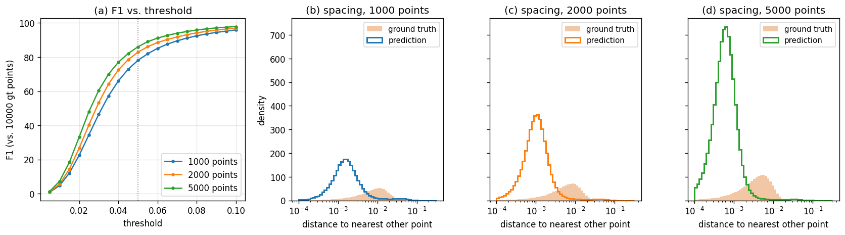
(a) F1 against the same 10k ground-truth points per chair. (b–d) Distance from each point to its nearest other point, for the prediction and for the same number of points sampled from the ground truth: the predicted points are much closer together, more so with more points.
- More points raise F1, but mostly through coverage: recall@0.05 goes from 77 to 90, precision only from 81 to 86. At small thresholds all models stay poor (F1@0.02 ≤ 33).
- The extra points bunch up more, not less: the spacing drops from 0.44× to 0.16× that of an even sample. With no one-to-one matching in chamfer, most new points land where points already are.
- Less of the score comes from the image: a single average chair with 5000 points already scores 77.4, so the gain from the image shrinks from +21.8 to +8.3.
- Conclusion: a denser cloud scores higher on F1@0.05 without being more detailed or more specific to the input.
Smoothness weight and mesh regularizers (2.3: can the folded surface be fixed?)
All runs start from the 2.3 model and change one thing. Surface quality: normal inconsistency (mean 1 − cos of the angle between adjacent faces; 0 = smooth).

| w_smooth | F1@0.05 | Normal inconsistency |
|---|---|---|
| 0 | 72.13 | 1.223 |
| 0.1 (2.3) | 70.41 | 0.290 |
| 1 | 68.22 | 0.104 |
| 10 | 58.26 | 0.021 |
(Only the ratio w_smooth / w_chamfer matters with Adam, so this also covers w_chamfer.)
- w_smooth only moves along a trade-off. Without smoothing the mesh is shredded into spikes but has the highest F1; with strong smoothing it is a clean blob with no legs and the lowest F1. No value gives both a clean surface and legs.

| Model | F1@0.05 | Normal inconsistency |
|---|---|---|
| 2.3 model | 70.41 | 0.290 |
| + edge length + normal consistency losses | 68.98 | 0.064 |
+ finer template ico_sphere(5) |
72.02 | 0.072 |
- Regularizers that target the actual failure fix it (as in Pixel2Mesh [5] and PyTorch3D's mesh-fitting tutorial [8]). An edge-length term stops triangles from stretching across empty space and a normal-consistency term stops neighbouring faces from folding; together they give a clean surface with separate legs, unlike a strong Laplacian, which flattens everything.
- A finer template (4× more vertices) recovers the F1 (72.0, as high as the shredded mesh) with a real surface.
- Conclusion: for meshes, F1@0.05 does not see surface quality; the best-scoring mesh is the worst surface.
2.5 Interpreting the models
Two questions, one for each failure seen above.
Why do thin parts disappear from the voxel predictions? The same prediction drawn at three probability thresholds:

The folding chair almost vanishes at p > 0.5 but its frame and legs are clearly there at p > 0.2. Over the test set, the mean predicted probability on occupied ground-truth voxels grows with how thick the part is (number of occupied neighbours out of 26):

| Occupied neighbours | 2 (thin rod) | 6 | 8 (thin board) | 17 (surface of a solid part) | 26 (inside) |
|---|---|---|---|---|---|
| Mean predicted probability | 0.15 | 0.17 | 0.25 | 0.39 | 0.53 |
The model does locate thin parts; it just gives them low probability. Thin parts are a tiny share of the occupied voxels (and only 4.3% of voxels are occupied), so BCE gains little from them and pushes them toward "empty".
Why do point and mesh predictions look alike for different chairs? Each predicted point is colored by its output index (by where that index lands on average), and each mesh vertex by its starting direction on the template sphere:

The same colors land on the same parts of every chair: for points, teal at the top of the backrest, pink at the legs; for the mesh, the green part of the sphere always becomes the backrest and the purple part the legs. Both decoders have learned one template chair with a fixed mapping from outputs to chair parts and deform it only slightly per image (median standard deviation of a point's position across test chairs: 0.07, for a chair about 1.0 tall).
What does each model do when it knows nothing? Given the mean training feature, the voxel decoder predicts an empty grid (BCE pushes uncertain voxels to the 96% "empty" prior), while the point and mesh decoders predict a generic average chair (chamfer pushes uncertain points to the middle of all plausible positions). This is the same behaviour as above at a smaller scale: voxel models drop what they are unsure about, point and mesh models blur it into an average.
3. Exploring other architectures / datasets
3.1 Implicit network
Input RGB, the 2.1 conv decoder, the implicit decoder queried at 32³ and at 128³ (same model), and the ground-truth mesh (all voxel models at isovalue 0.3, see below):

Model
An occupancy network [6]: f(feature, x, y, z) → occupancy logit, with (x, y, z) ∈ [−1, 1)³. The query point goes through a positional encoding [7] (sin/cos at 5 frequencies), is combined with the image feature in the first layer, and passes through a 4-layer MLP of width 256 (0.35M parameters).
- Training: BCE (as in 2.1) on 4096 random cells of the 32³ grid per chair per step. Each query point is jittered within its cell, so the function is also learned between grid points.
- Inference: query a full 32×32×32 meshgrid of (−1, 1)³, or any other resolution, and run marching cubes as in 2.1.
Evaluation
Threshold. At the default isovalue 0.5 the implicit model scores only 43.0, with 101 empty predictions. Its probabilities are flatter than the conv decoder's (its most confident voxel is about 0.69 for a typical chair, vs. 0.96), so a 0.5 threshold removes most of the shape. Both models do best at isovalue 0.3 on the validation set, so both are compared at 0.3:
| Model (isovalue 0.3) | Parameters | F1@0.05 |
|---|---|---|
| Conv voxel decoder (2.1) | 11.2M | 63.89 |
| Implicit, queried at 32³ | 0.35M | 62.38 |
| Implicit, queried at 128³ (same model) | 0.35M | 62.64 |

- Almost the same F1 as the conv decoder with 1/30 of the parameters.
- Any resolution from one model. At 128³ the surface is smooth (no 32³ staircase) at the same F1; it cannot add detail beyond the 32³ labels it was trained on.
- The shapes are rounder than the conv ones and lose more thin parts (the office chair's base becomes one stub, the folding chair is only its seat), and thin parts get the same low probability as with the conv decoder (≈0.16). Changing the decoder does not change how BCE treats rare thin parts.
3.2 Parametric network
Input RGB, the 2.2 MLP, the parametric model's points and mesh (colored by patch), and the ground-truth mesh:

Model
AtlasNet [4]: 8 MLPs g_k(feature, u, v) → (x, y, z), each folding the unit square onto part of the surface. Each patch: [feature, u, v] → 512 → 256 → 128 → 3 with ReLU (3.4M parameters in total).
- Training: every forward pass samples 125 random (u, v) per patch, giving 1000 points; the loss is the same chamfer loss as 2.2.
- Output: any number of points from one model, and a mesh for free by mapping a regular (u, v) grid per patch.
Evaluation
F1@0.05 = 72.85 (2.2 MLP: 76.26)

Against the same 10k ground-truth points per chair:
| Model | F1@0.01 | F1@0.02 | F1@0.05 | Spacing / ground truth |
|---|---|---|---|---|
| MLP, 1000 points (2.2) | 4.6 | 22.4 | 78.1 | 0.44 |
| Parametric, 1000 points | 5.1 | 24.3 | 74.5 | 0.70 |
| MLP, 5000 points (separate model, 2.4) | 7.2 | 33.1 | 86.1 | 0.16 |
| Parametric, 5000 points (same model) | 13.9 | 42.1 | 81.0 | 0.70 |
- Lower F1@0.05 but more accurate at small thresholds. The points lie on thin sheets close to the surface; the MLP's fuzzy cloud covers more of the chair within the lenient 0.05.
- Points spread more evenly (spacing 0.70× instead of 0.44×), and stay even when sampled with 5000 points: each patch is a continuous function of (u, v), so neighbouring samples land next to each other instead of on the same spot.
- 3 of the 8 patches collapsed to a single point (area ≈ 0), so 375 of the 1000 points sit on three spots; the other 5 patches cover the chair. Fewer patches or a term that keeps each patch's area up would avoid this.
3.3 Extended dataset for training
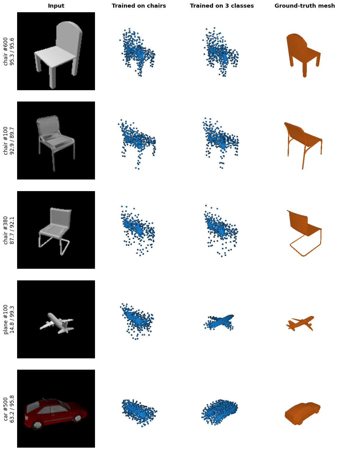
Input RGB, the 2.2 model trained on chairs only, the same model trained on chairs, cars and planes, and the ground-truth mesh. Three test chairs (the 2.2 examples), then a plane and a car; row labels give F1 for the chair-only / 3-class model:
Setup
dataset_location.py selects the 3-class dataset when R2N2_FULL=1 is set. I trained the 2.2 point-cloud model (1000 points, same settings and the same number of iterations) on chairs, cars and planes. The chair train/test lists of the 3-class split are identical to the chair-only split, so both models are compared on exactly the same 678 test chairs (same views).
Evaluation
| Test set | Trained on chairs | Trained on 3 classes |
|---|---|---|
| Chairs (678) | 76.15 | 77.06 |
| Cars (368) | 61.11 | 93.02 |
| Planes (405) | 42.02 | 95.72 |
| Diversity (prediction pair distance / ground-truth pair distance) | Trained on chairs | Trained on 3 classes |
|---|---|---|
| Chairs | 0.43 | 0.42 |
| Cars | 0.70 | 0.49 |
| Planes | 0.69 | 0.31 |
(F1@0.05. Diversity: for 500 random pairs of test shapes of one class, the distance between the two predictions divided by the distance between the two ground truths; lower = closer to a single template.)
- Chairs do not get worse, maybe slightly better (77.1 vs. 76.2; better on 351 of 678 chairs, close to an even split), although the 3-class model saw only about half as many chair images in the same training budget. Adding cars and planes did not take capacity away from chairs.
- Chair predictions look the same for both models (same fuzzy chair, same missing frame on #380) and are just as template-like (0.42 vs. 0.43). Training on more classes does not make the chair predictions more specific.
- The class comes from the image feature. The 3-class model gives planes wings and a tail and cars a box shape, and scores above 93 on both. The chair-only model puts a chair-shaped cloud on every input (plane #100: F1 14.8), so it scores 61 on cars and 42 on planes.
- Cars and planes score higher than chairs, partly because they vary less: their predictions are even closer to one template (0.49, 0.31) and still score above 93. Chairs differ much more in structure (legs, frames, holes), so a template fits them worse. Within each class, the 3-class model is consistent (one layout per class) but not very diverse.
References
- C. B. Choy, D. Xu, J. Gwak, K. Chen, S. Savarese. 3D-R2N2: A Unified Approach for Single and Multi-view 3D Object Reconstruction. ECCV 2016.
- A. X. Chang et al. ShapeNet: An Information-Rich 3D Model Repository. arXiv:1512.03012, 2015.
- H. Fan, H. Su, L. Guibas. A Point Set Generation Network for 3D Object Reconstruction from a Single Image. CVPR 2017.
- T. Groueix, M. Fisher, V. G. Kim, B. C. Russell, M. Aubry. AtlasNet: A Papier-Mâché Approach to Learning 3D Surface Generation. CVPR 2018 (arXiv:1802.05384).
- N. Wang, Y. Zhang, Z. Li, Y. Fu, W. Liu, Y.-G. Jiang. Pixel2Mesh: Generating 3D Mesh Models from Single RGB Images. ECCV 2018.
- L. Mescheder, M. Oechsle, M. Niemeyer, S. Nowozin, A. Geiger. Occupancy Networks: Learning 3D Reconstruction in Function Space. CVPR 2019 (arXiv:1812.03828).
- B. Mildenhall, P. P. Srinivasan, M. Tancik, J. T. Barron, R. Ramamoorthi, R. Ng. NeRF: Representing Scenes as Neural Radiance Fields for View Synthesis. ECCV 2020.
- N. Ravi et al. Accelerating 3D Deep Learning with PyTorch3D. arXiv:2007.08501, 2020.
- K. He, X. Zhang, S. Ren, J. Sun. Deep Residual Learning for Image Recognition. CVPR 2016.