16-825 Assignment 4: Multi-View Transformers
1. Multi-View Data Preprocessing
1.1–1.2 Unprojection (original world frame, meters)
Command: python scripts/visualize_data.py --stage unprojection --num-scenes 5 --max-points 10000.
Each view's depth is unprojected with its resized intrinsics and original camera-to-world pose, so all
views should form one consistent point cloud in the ScanNet++ world frame.

1.3 Canonicalization
Command: python scripts/visualize_data.py --stage canonicalization --num-scenes 5 --max-points 10000.
After canonicalization camera 0 sits at the origin with identity pose, and the valid-point centroid is
1 unit from the origin.

Canonical first-view coordinates. First camera center (X, Y, Z): (0.0000, 0.0000, 0.0000) normalized units. Scene scale: 1.867 m. Valid-point centroid distance: 1.000 normalized units. The red frustum marks the first sampled camera; black depth pixels indicate missing measurements.
1.7 Final check
Command: python scripts/check_data.py --config configs/scannetpp/iphone/data.json --split train --max-samples 4.
All four samples have 8 views at 224×224, reprojection errors around 10−4 px
(requirement: < 0.01 px) and a centroid distance of 1.
| Sample | Valid depth | Max point reproj. error (px) | Max ray reproj. error (px) | Centroid distance |
|---|---|---|---|---|
e050c15a8d_frame_007080 | 0.978 | 1.10e-4 | 1.08e-4 | 1.000 |
5f99900f09_frame_002820 | 0.990 | 1.23e-4 | 1.11e-4 | 1.000 |
47b37eb6f9_frame_002720 | 0.961 | 9.88e-5 | 8.90e-5 | 1.000 |
4c5c60fa76_frame_006690 | 0.752 | 1.13e-4 | 1.02e-4 | 1.000 |
Full check_data.py output
{
  "split": "train",
  "dataset_samples": 224,
  "checked_samples": 4,
  "samples": [
    {"sequence_name": "e050c15a8d_frame_007080", "views": 8, "resolution": 224,
     "valid_depth_fraction": 0.9779127240180969,
     "max_reprojection_error_px": 0.00011009880108758807,
     "max_ray_reprojection_error_px": 0.00010764275066321716,
     "centroid_distance": 1.0},
    {"sequence_name": "5f99900f09_frame_002820", "views": 8, "resolution": 224,
     "valid_depth_fraction": 0.9903116226196289,
     "max_reprojection_error_px": 0.00012302029062993824,
     "max_ray_reprojection_error_px": 0.00011108566104667261,
     "centroid_distance": 0.9999999403953552},
    {"sequence_name": "47b37eb6f9_frame_002720", "views": 8, "resolution": 224,
     "valid_depth_fraction": 0.9609947800636292,
     "max_reprojection_error_px": 9.881925507215783e-05,
     "max_ray_reprojection_error_px": 8.897326188161969e-05,
     "centroid_distance": 1.0},
    {"sequence_name": "4c5c60fa76_frame_006690", "views": 8, "resolution": 224,
     "valid_depth_fraction": 0.7516716122627258,
     "max_reprojection_error_px": 0.00011280165199423209,
     "max_ray_reprojection_error_px": 0.00010225349979009479,
     "centroid_distance": 0.9999999403953552}
  ],
  "batch_shapes": {
    "rgb": [2, 8, 3, 224, 224], "depth": [2, 8, 1, 224, 224], "depth_valid": [2, 8, 1, 224, 224],
    "K": [2, 8, 3, 3], "frame_numbers": [2, 8], "T_world_from_camera": [2, 8, 4, 4],
    "original_world_from_reference": [2, 4, 4], "scene_scale": [2],
    "points_world": [2, 8, 3, 224, 224], "ray_origins": [2, 8, 3, 224, 224],
    "ray_directions": [2, 8, 3, 224, 224], "plucker": [2, 8, 6, 224, 224]
  }
}
Explanations
Canonicalization. I express all camera poses relative to the first sampled camera using
T′i = Tworld←0−1Tworld←i, computed in float64.
This makes camera 0 the identity. I then unproject the valid depth pixels in this reference frame and compute
s = ‖mean(valid points)‖. Dividing translations, depth and points by the same scale preserves their geometry
and places the valid-point centroid one unit from the origin. Rotations and intrinsics stay unchanged, and I do not subtract
the centroid. This gives every sample a consistent reference frame and scale, reducing the ambiguity in supervision.
World-space ray directions. For pixel (u, v),
K−1[u, v, 1]T gives a camera-space direction with z-coordinate 1.
Multiplying this vector by optical-axis z-depth produces the camera-space point. To construct a ray, I rotate the direction
with the camera-to-world rotation and normalize it:
d = normalize(RK−1[u, v, 1]T).
The ray origin is the camera center, o = t. Translation changes the origin but does not change the direction.
Plücker moment. I encode each ray as [d, m], where
m = o × d. Any point p = o + λd on the same line gives the same moment because
p × d = o × d. The encoding therefore represents an oriented line independently of the chosen
point along it. For a unit direction, ‖m‖ is the line’s distance from the world origin.
Together, direction and moment describe the viewing line in the canonical frame.
2.1 Mini-LVSM Overfitting
Command: python -m models.lvsm.train --overfit 2000 --output-dir outputs/lvsm_overfit
(2000 steps on one fixed batch of 4 samples, 2 source + 6 target views each; 768 s on an NVIDIA A10G).
Final overfit PSNR on the fixed batch: 31.06 dB (SSIM 0.873, MSE 8.4e-4). The epoch-average training PSNR over all 2000 steps was 25.48 dB.

val_epoch000.png after overfitting. Columns: source 1, source 2, ground-truth target, prediction.2.2 Mini-LVSM Training and Evaluation
Training settings
- Model: 14.6M parameters, patch size 8 (784 tokens per 224×224 view), width 384, 8 transformer blocks,
head dim 64 (6 heads), MLP ratio 4, QK-norm. Each target is rendered from a sequence of
(S+1)×784tokens with full bidirectional attention. - Data: 8 views per sample from a 32-frame window,
num_source_views = 2(6 targets per sample), batch size 4, 224 training scenes (56 steps/epoch). - Optimization: 100 epochs (5,600 steps), AdamW (lr 2e-4, weight decay 0.05, betas 0.9/0.95), 200 warmup steps followed by cosine decay to 10% of the peak, gradient clipping 1.0, bfloat16 autocast with the MSE loss in float32.
- Hardware: one NVIDIA A10G (AWS g5.2xlarge), about 28 s/epoch (~47 min total).
Training curves

outputs/lvsm/log.jsonl).
The final checkpoint is also the best: validation PSNR 16.14 dB, SSIM 0.560.Training and validation PSNR continue to improve near epoch 100, suggesting that the model may benefit from additional training. Validation PSNR is slightly higher than training PSNR. One possible reason is that training metrics average predictions made throughout an epoch, whereas validation uses the updated weights at its end. The sampling procedures also differ: training uses random windows, while validation uses fixed views from the first 32 frames.
Training visualizations


Columns in every LVSM visualization: source views, ground-truth target, prediction.
Ablation: number of source views × target-ray conditioning
Command: python -m models.lvsm.eval --checkpoint outputs/lvsm/best.pt --num-source-views 1 2 4 --conditioning correct shuffled none
(28 validation scenes, 8 views from the first 32 frames, seed 825).
| Source views | correct | shuffled | none | Target images | |||
|---|---|---|---|---|---|---|---|
| PSNR ↑ | SSIM ↑ | PSNR ↑ | SSIM ↑ | PSNR ↑ | SSIM ↑ | ||
| S = 1 | 15.20 | 0.558 | 11.80 | 0.487 | 12.47 | 0.529 | 196 |
| S = 2 (trained) | 16.14 | 0.560 | 11.48 | 0.472 | 12.45 | 0.528 | 168 |
| S = 4 | 16.86 | 0.575 | 11.60 | 0.474 | 12.47 | 0.538 | 112 |
Evaluation visualizations

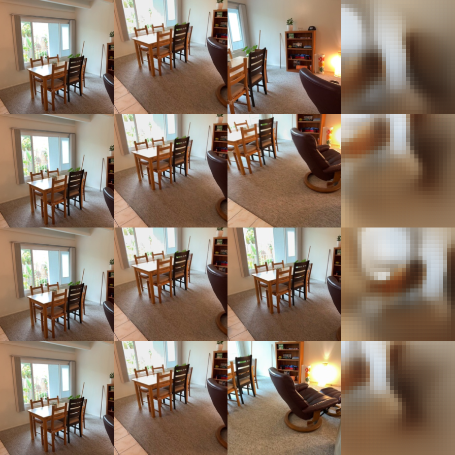
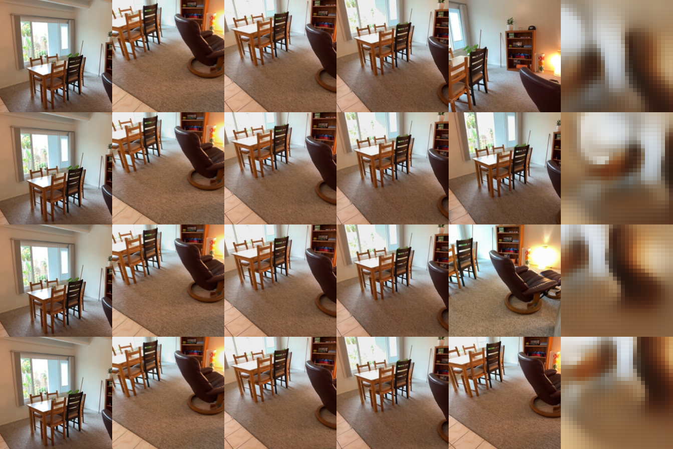

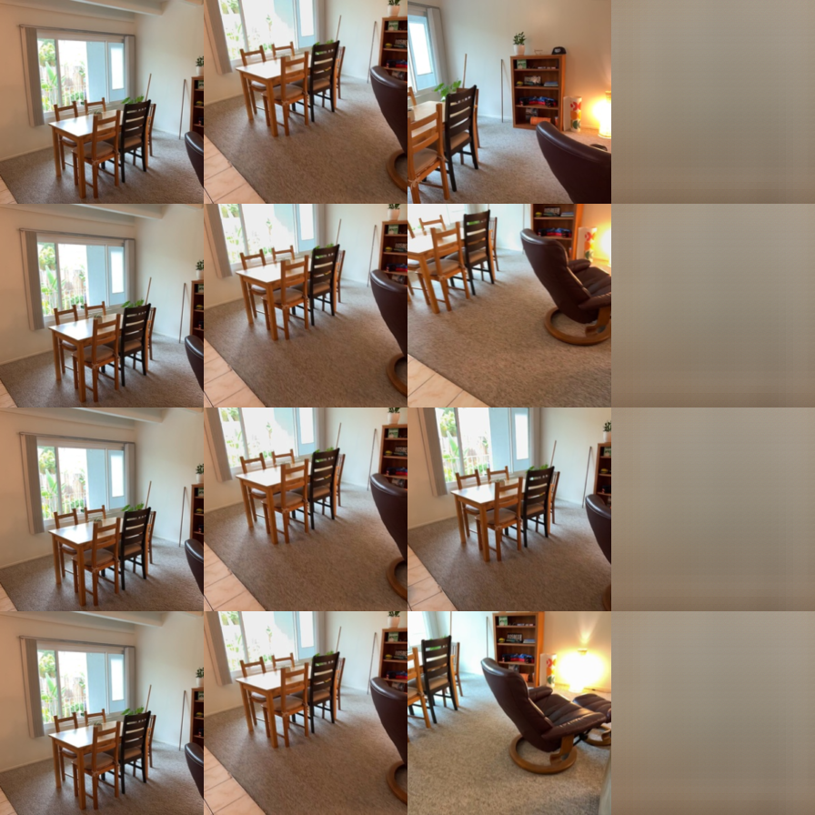
All nine ablation images


Discussion
Number of source views. With correct target rays, PSNR increases from 15.20 to 16.14 to 16.86 dB as the number of sources increases from 1 to 2 to 4. SSIM also increases, from 0.558 to 0.560 to 0.575. Additional views can provide coverage of regions that are occluded in a single source. Although the model was trained with S = 2, its attention layers accept different source-token counts at evaluation. However, this is not a comparison on a fixed target set: increasing S reduces the number of evaluated targets from 196 to 168 to 112, which may also affect the scores.
Ray conditioning. Shuffling or removing target rays reduces PSNR by roughly 3–5 dB relative to correct conditioning. Under either ablation, adding source views provides little benefit. This supports the conclusion that the model uses target rays to choose the rendered viewpoint. Zero rays produce predictions with little spatial detail; shuffled rays provide a different target camera and can produce structure that is misaligned with the ground truth. The lower scores for shuffled rays are consistent with MSE penalizing misplaced structure more strongly than a smooth prediction.
Limitations. Predictions capture coarse room layout and color but remain blurry and show 8×8 patch artifacts. Fine textures are poorly reconstructed. The model has only 14.6M parameters and was trained for 5,600 steps using MSE alone. Limited training and the averaging encouraged by MSE are plausible contributors, although these experiments do not isolate their individual effects.
2.3 Bonus: Training with a Random Number of Source Views
Question
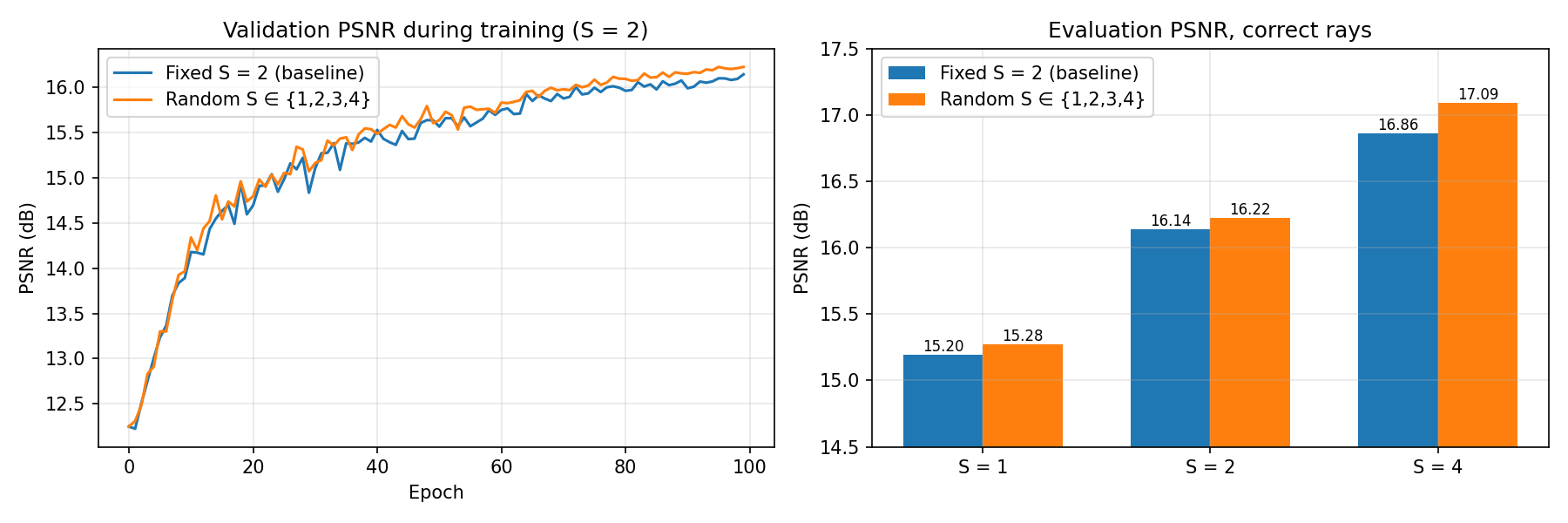
The baseline is trained only with S = 2 source views but evaluated with 1, 2 and 4. Does training with a random number of source views each step make the model better at handling different source counts at test time?
Setup
Controlled comparison: the only change is that each training step samples S uniformly from {1, 2, 3, 4} (torch RNG,
same seed), so each step has T = 8 − S targets. Model, data, batch size, 100 epochs, optimizer, schedule
and validation (S = 2) are identical to Q2.2. Config: configs/lvsm_random_s.json
("source_views_range": [1, 4]), implemented in train_one_epoch. I evaluated both runs' best.pt
(epoch 99 for both) with the same ablation command as Q2.2. Training took 29.3 s/epoch vs. 28.2 s/epoch for the baseline.
| Source views | correct rays: PSNR ↑ / SSIM ↑ | shuffled: PSNR | none: PSNR | ||||
|---|---|---|---|---|---|---|---|
| Fixed S = 2 | Random S | Δ PSNR | Fixed | Random | Fixed | Random | |
| S = 1 | 15.20 / 0.558 | 15.28 / 0.559 | +0.08 | 11.80 | 11.76 | 12.47 | 12.49 |
| S = 2 | 16.14 / 0.560 | 16.22 / 0.560 | +0.08 | 11.48 | 11.43 | 12.45 | 12.46 |
| S = 4 | 16.86 / 0.575 | 17.09 / 0.575 | +0.23 | 11.60 | 11.47 | 12.47 | 12.48 |
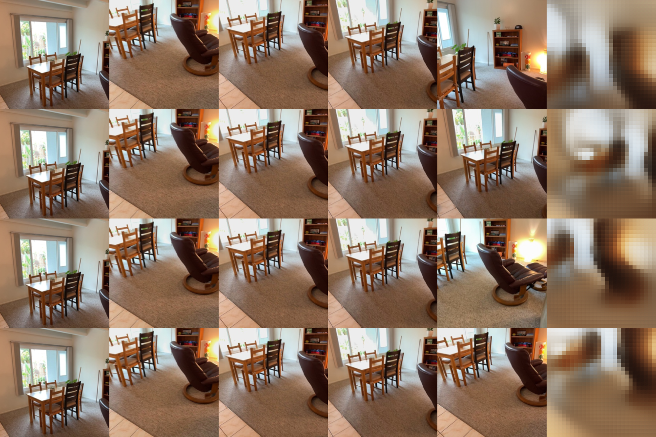
Findings
- Small, consistent gains with correct rays: +0.08 dB at S = 1 and S = 2, and +0.23 dB at S = 4. The largest gain is at S = 4, which the baseline never saw in training. Exposure to several source counts may help the model combine additional source tokens, although this single run does not establish the cause. SSIM is essentially unchanged (within ±0.001).
- No cost at the trained setting: even at S = 2, where the baseline trains every step, the random-S model is slightly better, although on average it sees fewer target images per step (5.5 vs. 6). Its validation curve stays slightly above the baseline for most of training.
- Slightly more reliant on the rays: with shuffled rays, random-S is a bit worse than the baseline (down to −0.13 dB at S = 4), and zero rays give the same result. This is consistent with greater sensitivity to target-ray conditioning, but the differences are too small to establish that explanation.
- Visually the outputs look almost the same: both are still blurry with 8×8 patch artifacts, so the gains are mostly in coarse color and layout accuracy.
Conclusion and limitations
Randomizing the number of source views during training is a cheap change (about 4% slower) that gives a small, consistent improvement, largest at S = 4, a source count absent from baseline training. However, the effects are small (0.1–0.2 dB), and each configuration was trained once with one seed, so part of the difference could be run-to-run noise. Several seeds would be needed to confirm it. The source counts were also limited to 1–4, and as in Q2.2, the number of target images differs between S settings.
3.1 Mini-VGGT Overfitting
Command: python -m models.vggt.train --config configs/vggt.json --overfit --output outputs/vggt_overfit
I trained on one fixed eight-view clip for 40 epochs with 25 steps per epoch (1,000 updates), using a learning rate of 1e-3. The fixed-clip evaluation loss decreased from 5.483 before training to −0.166. Depth AbsRel decreased from 0.619 to 0.0365, while δ1 increased from 0.208 to 0.956. Mean rotation and translation-direction errors fell to 0.344° and 0.442°, respectively. These metrics indicate that the model can fit the clip. The screenshot below compares ground-truth and predicted geometry.
The depth objective includes a confidence term, c|e| − 0.2 log(c), so a negative loss is possible.
It should be interpreted alongside depth and camera accuracy rather than as a nonnegative reconstruction error.


3.2 Mini-VGGT Training and Evaluation
Training settings
I used a frozen DINOv2 ViT-B/14 encoder with eight frame/global attention pairs, width 384 and six heads. Each training sample contains eight 224×224 views sampled from a 32-frame window. Training used all 224 scenes, a batch size of 16 and 1,000 epochs (14 updates per epoch). AdamW used a peak learning rate of 6e-4 and weight decay 0.01, with 10 warmup epochs followed by cosine decay to 5% of the peak. The total objective weights camera loss by 5 and depth loss by 1. The run used bf16 precision on one NVIDIA A10G. Summed epoch times in the training log total approximately 5.83 hours.
Loss curve

Metrics (8 views from the first 32 frames, 224px, seed 825)
| Split | AbsRel ↓ | δ1 ↑ | Rotation AUC ↑ | Translation AUC ↑ | Joint pose AUC ↑ | ||||||
|---|---|---|---|---|---|---|---|---|---|---|---|
| @5° | @15° | @30° | @5° | @15° | @30° | @5° | @15° | @30° | |||
| Val | 0.157 | 0.796 | 0.220 | 0.558 | 0.725 | 0.013 | 0.081 | 0.196 | 0.004 | 0.066 | 0.178 |
| Test | 0.164 | 0.778 | 0.234 | 0.562 | 0.743 | 0.016 | 0.094 | 0.209 | 0.004 | 0.067 | 0.187 |
Evaluated outputs/vggt_train/best.pt (epoch 929, lowest validation loss) on the full splits (28 scenes each, 784 view pairs, no degenerate pairs).
Numbers from outputs/vggt_train/metrics.json (val) and outputs/vggt_train/test_metrics.json (test).
GT vs. predicted geometry (four held-out scenes)
Scene 1: 09c1414f1b


Scene 2: 21d970d8de


Scene 3: 280b83fcf3


Scene 4: 2b1dc6d6a5


Each row compares GT (left) and prediction (right) for the same scene. Click an image to inspect it at full size. Screenshots come from outputs/vggt_train/visualization/index.html.
Discussion
Held-out depth accuracy is similar across splits: AbsRel is 0.157 on validation and 0.164 on test, while δ1 is 0.796 and 0.778. Test depth is slightly worse, but the gap is small in this evaluation. Rotation is substantially more accurate than translation direction: at 30°, validation AUC is 0.725 for rotation and 0.196 for translation. Joint pose AUC is only 0.178, indicating that translation remains a major limitation. Test pose AUC is slightly higher at 0.187, so the test split is not uniformly harder across tasks.
These aggregate metrics do not identify which surfaces or scenes cause the largest errors. Compared with GT, the dining-room prediction smooths the table and chair boundaries, while the hallway prediction loses some of the sharper wall structure. The office reconstruction is more diffuse around the chair and desk. These examples show that coarse layout is recovered more reliably than fine geometry; they do not isolate the causes of the errors.
3.3 Bonus: Number of Input Views at Evaluation
Question
Mini-VGGT was trained with exactly 8 views. How do accuracy, runtime and memory change if the same model is given fewer or more views at test time?
Setup
I evaluated the Q3.2 checkpoint (outputs/vggt_train/best.pt, no retraining) on the full validation split
with V = 2, 4, 8, 16 and 32 views. Everything else matches the Q3.2 evaluation: views come from the first 32 prepared
frames with seed 825, at 224px, and metrics use the same evaluate function. Runtime is the average forward
pass per scene (batch size 1, bf16, after two warm-up scenes) on one NVIDIA A10G. Memory is the peak allocated GPU
memory during those forward passes. Script: scripts/vggt_num_views.py.
| Views | AbsRel ↓ | δ1 ↑ | Rot AUC@30 ↑ | Trans AUC@30 ↑ | Pose AUC@30 ↑ | Pose pairs | ms / scene | Peak GPU memory |
|---|---|---|---|---|---|---|---|---|
| 2 | 0.122 | 0.852 | 0.732 | 0.176 | 0.160 | 28 | 42.7 | 0.74 GB |
| 4 | 0.135 | 0.849 | 0.727 | 0.213 | 0.192 | 168 | 41.0 | 0.76 GB |
| 8 (trained) | 0.157 | 0.796 | 0.726 | 0.196 | 0.178 | 784 | 43.8 | 0.81 GB |
| 16 | 0.186 | 0.747 | 0.711 | 0.179 | 0.164 | 3360 | 58.3 | 0.89 GB |
| 32 | 0.195 | 0.714 | 0.707 | 0.160 | 0.145 | 13888 | 113.8 | 1.05 GB |

Findings
- Depth gets steadily worse with more views: AbsRel 0.122 → 0.195 and δ1 0.852 → 0.714 from 2 to 32 views. All views share one normalized scale, set by camera 0 and the centroid of all valid points. Changing the view count also changes the selected frames and the geometry used to compute scale, so this experiment does not isolate the effect of additional context. These changes may contribute to the depth trend. At V > 8 the global attention also sees more tokens than in training.
- Camera accuracy is best near the training setting. Rotation AUC barely changes (0.73 → 0.71). Translation and joint pose AUC peak at V = 4–8 and fall for 16 and 32 views, which are outside the training distribution. With only 2 views there is a single pair per scene (28 pairs in total), so the V = 2 camera numbers are noisy.
- Runtime is flat up to 8 views, then grows quickly: about 42 ms up to V = 8, then 58 ms at 16 and 114 ms at 32.
The nearly flat timing at small V suggests that fixed overhead or limited GPU utilization may dominate; profiling would be needed to confirm this. At large V, the per-frame work grows linearly, and
global attention over
V·261tokens grows quadratically. Doubling from 16 to 32 views nearly doubles the time. - Memory grows only slightly (0.74 → 1.05 GB), which is consistent with inference avoiding saved backward activations and using memory-efficient attention. The reported peak includes model weights and forward-pass allocations; a memory breakdown would be needed to identify the dominant component.
Conclusion and limitations
A model trained with a fixed number of views does not automatically get better with more views: per-view depth degrades, and camera accuracy is best near the training count. Training with a variable or larger view count is a possible follow-up, but this evaluation does not test whether it would improve accuracy. Limitations: one checkpoint, validation split only, evaluation-time changes only (no retraining), and every setting draws views from the same 32-frame window. That means V = 32 uses every frame, with many nearly identical neighboring views, and the number of pose pairs varies widely between settings.
3.3 Bonus (second exploration): Point-Map Prediction and Multi-Task Synergy
Questions
- Does a direct point-map head produce more accurate 3D points than unprojecting predicted depth with predicted cameras?
- Does learning cameras and depth jointly, or adding point maps as a third task, help each task compared with training it alone?
Setup
I trained three additional models with the Q3.2 configuration (frozen DINOv2 ViT-B/14, 8 views, sampling range 32, batch size 16, 1,000 epochs, same optimizer and schedule). Each run changes only the loss configuration:
| Run | Loss weights (camera / depth / points) | Config | Best epoch |
|---|---|---|---|
| Joint (Q3.2) | 5 / 1 / – | configs/vggt.json | 929 |
| Joint + points | 5 / 1 / 1 | configs/vggt_points.json | 912 |
| Camera only | 5 / 0 / – | configs/vggt_camera_only.json | 715 |
| Depth only | 0 / 1 / – | configs/vggt_depth_only.json | 839 |
The point head mirrors the depth head: a linear patch decoder to a 3-channel (x, y, z) map in the
canonical first-camera frame, followed by an RGB-conditioned residual CNN, with no output activation. The point loss
is the trimmed mean of the per-pixel Euclidean error on GT-valid pixels, plus the depth gradient loss averaged over the
three coordinates. In the single-task runs, the other head still exists but receives no gradient, so its metrics are
not meaningful and are shown as “–”. Each best.pt is selected by the lowest validation loss of that
run's own objective and evaluated exactly as in Q3.2. 3D point error is the mean Euclidean distance to the GT point map over
GT-valid pixels, in normalized units and in meters (scripts/vggt_points_eval.py). The joint + points run took
about 23.1 s per epoch versus 20.7 s for the single-task runs.
Multi-task comparison
| Run | Validation | Test | ||||||||
|---|---|---|---|---|---|---|---|---|---|---|
| AbsRel ↓ | δ1 ↑ | Rot@30 ↑ | Trans@30 ↑ | Pose@30 ↑ | AbsRel ↓ | δ1 ↑ | Rot@30 ↑ | Trans@30 ↑ | Pose@30 ↑ | |
| Joint (Q3.2) | 0.157 | 0.796 | 0.725 | 0.196 | 0.178 | 0.164 | 0.778 | 0.743 | 0.209 | 0.187 |
| Joint + points | 0.136 | 0.839 | 0.684 | 0.166 | 0.150 | 0.152 | 0.806 | 0.718 | 0.197 | 0.183 |
| Camera only | – | – | 0.710 | 0.189 | 0.169 | – | – | 0.715 | 0.164 | 0.145 |
| Depth only | 0.152 | 0.806 | – | – | – | 0.175 | 0.766 | – | – | – |
AUC at 5° / 15° / 30° (test)
| Run | Rotation AUC | Translation AUC | Joint pose AUC |
|---|---|---|---|
| Joint (Q3.2) | 0.234 / 0.562 / 0.743 | 0.016 / 0.094 / 0.209 | 0.004 / 0.067 / 0.187 |
| Joint + points | 0.202 / 0.523 / 0.718 | 0.008 / 0.073 / 0.197 | 0.002 / 0.055 / 0.183 |
| Camera only | 0.207 / 0.516 / 0.715 | 0.010 / 0.065 / 0.164 | 0.001 / 0.038 / 0.145 |
3D point accuracy: direct point map vs. cameras + depth
| Model | Points from | Val error (normalized / m) | Test error (normalized / m) |
|---|---|---|---|
| Joint (Q3.2) | predicted cameras + predicted depth | 0.289 / 0.580 | 0.245 / 0.480 |
| Joint + points | predicted cameras + predicted depth | 0.264 / 0.534 | 0.231 / 0.451 |
| Joint + points | direct point head | 0.275 / 0.560 | 0.239 / 0.463 |
| Joint (Q3.2) | GT cameras + predicted depth | 0.157 / 0.337 | 0.153 / 0.315 |
| Joint + points | GT cameras + predicted depth | 0.137 / 0.298 | 0.147 / 0.294 |
The GT-camera rows are diagnostic only: they use ground-truth cameras to isolate the error that comes from depth.

09c1414f1b.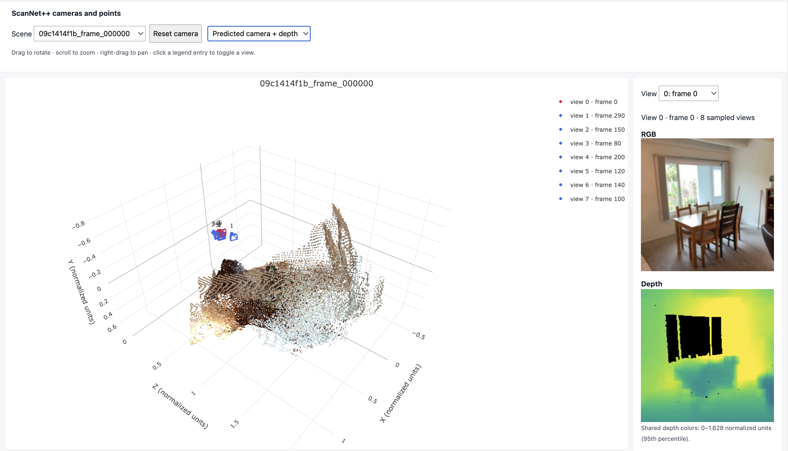
09c1414f1b.
09c1414f1b.All three screenshots show the same dining-room scene. Both prediction paths recover the broad layout, but the point clouds are more diffuse than GT and fine furniture structure is less distinct. This example illustrates reconstruction differences; the split-wide metrics above provide the quantitative comparison. Click an image to inspect it at full size.
Findings
- The direct point map is close to, but slightly less accurate than, unprojection from the same model: 0.275 vs. 0.264 on validation and 0.239 vs. 0.231 on test. Both are more accurate than the Q3.2 joint model's camera+depth points (0.289 and 0.245). In this setup, the point head does not outperform the camera+depth path.
- Camera error appears to be the largest contributor to 3D point error. Replacing predicted cameras with GT cameras roughly halves the error for both models (for example, 0.289 → 0.157 on validation for the joint model). This diagnostic uses GT cameras, so it indicates where the error comes from rather than an achievable result.
- Adding point supervision improved depth but reduced camera accuracy. AbsRel decreased from 0.157 to 0.136 (val) and from 0.164 to 0.152 (test), while pose AUC@30 decreased from 0.178 to 0.150 (val) and from 0.187 to 0.183 (test). One possible explanation is competition between objectives for the shared transformer; this experiment does not test that explanation.
- Depth supervision appears to help camera estimation. The camera-only model is worse than the joint model on both splits, most clearly on test (translation AUC@30 0.164 vs. 0.209; pose AUC@30 0.145 vs. 0.187). The validation gap is smaller (pose AUC@30 0.169 vs. 0.178).
- The effect of camera supervision on depth is inconclusive. The depth-only model is slightly better than the joint model on validation (AbsRel 0.152 vs. 0.157) but worse on test (0.175 vs. 0.164).
Conclusion and limitations
Under this training budget, joint camera and depth learning appears to benefit camera estimation, while its effect on depth is mixed across splits. A direct point-map head achieves 3D accuracy similar to unprojection, and adding it as an auxiliary task improves depth at some cost to camera accuracy. Limitations: each configuration was trained once with one seed, each split has only 28 scenes, the point loss weight (1.0) was not tuned, and each run's best checkpoint was selected by a different objective. Differences of a few thousandths may therefore fall within run-to-run variation.