16-825 Assignment 2: Single View to 3D
All training was done on an Apple GPU (--device mps) with the ResNet18 image
encoder. I did not use --load_feat.
1. Exploring Loss Functions
1.1 Fitting a Voxel Grid
Loss: binary cross-entropy on logits (binary_cross_entropy_with_logits). The source grid
is optimised for 3,000 steps, and occupancy is read out as logit ≥ 0 (probability ≥ 0.5).

1.2 Fitting a Point Cloud
Chamfer loss written from scratch: all pairwise squared distances, then the mean nearest-neighbour distance in both directions (source→target + target→source). 500 points, lr 0.01, 3,000 steps.

The fitted cloud looks sparser than the target even though both have 500 points. After fitting, the 500 source points occupy only 199 distinct locations (rounded to 0.001). Chamfer loss lets several source points collapse onto the same target point: the source→target term is satisfied as soon as each source point reaches some target point, and nothing in the loss pushes coincident points apart.
1.3 Fitting a Mesh
A level-4 ico-sphere is deformed with chamfer loss on 500 sampled surface points plus uniform Laplacian
smoothing (w_smooth = 0.1), lr 0.01, 3,000 steps.

2. Reconstructing 3D from a Single View
All models share the ResNet18 encoder (512-d feature) and are trained for 2,000 iterations with lr 4e-4. Unless noted, the batch size is 8.
Evaluation protocol. The test loader picks a random input view per chair, and the
F1 metric samples random surface points. I added a --seed flag to
eval_model.py, and every score on this page uses --seed 0. All models are
therefore scored on the same input view of each of the 678 test chairs, which makes per-chair comparisons
between models possible (used in 2.4 and 2.5). The figures in 2.1–2.3 show the same three test
chairs and views for every representation.
| Representation | Decoder | Decoder params | F1@0.05 |
|---|---|---|---|
| Voxel 32³ | Linear(512,1024) → ReLU → Linear(1024,32³) | 34.1 M | 41.58 |
| Point cloud, 1,000 points | Linear(512,1024) → ReLU → Linear(1024,3000) | 3.60 M | 73.31 |
| Mesh, level-4 ico-sphere | Linear(512,1024) → ReLU → Linear(1024,2562×3) | 8.40 M | 68.82 |
2.1 Image to Voxel Grid
The decoder outputs B×1×32×32×32 logits and is trained with BCE. At
evaluation, sigmoid is applied before marching cubes at isovalue 0.5.
F1@0.05 = 41.58


The voxel model captures the rough size and placement of each chair but produces rounded blobs. Thin parts are lost: in example 1 the lounge chair's thin frame disappears and only a small fragment of the seat survives. Only ~3% of voxels are occupied, so the unweighted BCE pushes uncertain regions toward “empty”. 14 of the 678 test chairs score exactly 0, typically because no voxel reaches probability 0.5 and the extracted surface is empty.
2.2 Image to Point Cloud
The decoder outputs 1,000 points and is trained with my chamfer loss.
F1@0.05 = 73.31


The point model scores highest, but its predictions are fuzzy shells with uneven density and a few dense clumps, rather than clear chair parts. The cloud covers the right volume, which is enough for the 0.05 threshold, but F1 falls quickly at 0.01–0.02 because few points lie exactly on the surface.
Continuing this model to 6,000 iterations (lr lowered to 1e-4 after step 2,000) raises F1@0.05 to 78.17 and improves 76% of the test chairs. To keep the comparison fair, every other number on this page uses the 2,000-iteration model, the same budget as the other representations.
2.3 Image to Mesh
The decoder predicts per-vertex offsets of a level-4 ico-sphere. Its last layer is zero-initialised, so training starts from the sphere. Loss = chamfer (1,000 sampled points) + 0.1 × Laplacian smoothing.
F1@0.05 = 68.82


The predicted meshes have stretched, spiky faces even though their sampled-surface F1 is fairly high.
Comparison: point cloud vs. mesh vs. voxel
Ranking: point cloud (73.31) > mesh (68.82) > voxel (41.58). The F1 metric compares points sampled on surfaces, so the more directly a representation is optimised for surface positions, the better it does:
- Point cloud is trained with chamfer distance, which is nearly the metric itself, and each point can move freely. Nothing forces the points to form a coherent surface, which is why it scores well but looks scattered.
- Mesh is also trained with chamfer loss, but every vertex is tied to a sphere's connectivity. A genus-0 sphere cannot open holes for the gaps between the chair's legs and back, so it stretches faces across them. Those spikes and sheets cost precision.
- Voxel is trained with a per-cell classification loss rather than a surface loss. It is limited to a 32³ grid, and the surface depends on the 0.5 threshold. Thin legs and slats are narrower than a cell or fall below the threshold, so they disappear and recall drops sharply.
2.4 Effect of Hyperparameters: Smoothness Weight
I retrained the mesh model with w_smooth = 1.0 (10× the baseline), keeping everything
else the same (w_chamfer 1.0, 1,000 points, batch size 8, lr 4e-4, 2,000 iterations).
| w_smooth | F1@0.01 | F1@0.02 | F1@0.03 | F1@0.04 | F1@0.05 |
|---|---|---|---|---|---|
| 0.1 (baseline) | 4.07 | 21.32 | 41.54 | 57.42 | 68.82 |
| 1.0 | 3.93 | 20.60 | 40.33 | 55.59 | 66.48 |
Because both models were evaluated with the same seed, every test chair is seen from the same view by both, so the scores can be compared chair by chair. The baseline is better by 2.34 F1@0.05 on average (paired 95% CI 1.79 to 2.90) and wins on 63% of the 678 chairs. It is also better at every distance threshold. So the drop is not evaluation noise, although each setting was still trained only once.


A stronger smoothness term makes the surfaces rounder and removes the sharpest spikes. The major artifacts (sheets spanning the gaps, missing chair structure) remain. Smoothing alone cannot fix the underlying problem, which is the fixed sphere topology. It only trades local sharpness for a consistently worse fit.
2.5 Interpreting the Model
I used four visualizations to look past the average F1. All of them use the 2,000-iteration models and the seeded evaluation, so every model sees the same view of every chair.
(a) Are the same chairs hard for every representation?

| Pair | Correlation of per-chair F1 | Shared chairs in both bottom 10% (of 67) |
|---|---|---|
| point – mesh | 0.80 | 41 |
| mesh – voxel | 0.18 | 19 |
| point – voxel | 0.06 | 13 |
The point and mesh models agree strongly on which chairs are hard. Both regress surface positions
with chamfer loss from the same kind of global feature, so they fail on the same inputs. The voxel model's
difficulty is almost unrelated to theirs, which points to a different failure mode. Its distribution is
also bimodal: a large group of chairs near F1 20 (blobs that miss the thin parts) and a second group that
works reasonably well. Part of the difference is the evaluation itself: for voxels, eval_model.py
re-centres both the predicted and the ground-truth points before comparing them, so voxel scores ignore
position errors. That turns out to matter, as (b) shows.
(b) Why do the worst point-cloud predictions fail?


The best and worst predictions look surprisingly alike: a fuzzy, roughly chair-sized cloud centred near the origin. What separates them is mostly where the ground truth is. ShapeNet chairs are not all centred at the origin. For chairs 71 and 491, the ground-truth bounding box is centred about 0.2 above it, but the model still predicts a cloud around the origin, which is four times the 0.05 threshold away. Across all test chairs, F1 correlates with this centre offset (r = −0.49). The worst 10% of chairs have a median offset of 0.143, against 0.072 for the rest. A single image cannot reveal an object's offset in the canonical frame, so the model learns to predict the average position. The bench (chair 510) is the exception: it is centred correctly but its long, low shape is far from the average chair.
(c) What does the learned feature space look like?

Blending the image features of two very different inputs gives a smooth morph from a tall, narrow cloud to a low, wide one, with no sudden jumps or broken shapes in between. The decoder has learned a continuous shape space whose main axes are coarse proportions (height, width, depth). It has not learned discrete parts: no intermediate step “removes the back” or “adds a crossbar”, which matches the blob-like predictions in 2.2.
(d) Does the prediction depend on the input view?
I fed four different views of the same held-out chair to the point-cloud model. For each view, the table gives F1@0.05 against the ground truth (using identical target samples) and the chamfer distance to the prediction from view 0.
| View | F1@0.05 | Chamfer to view-0 prediction |
|---|---|---|
| 0 | 47.40 | 0 |
| 2 | 46.74 | 0.00020 |
| 5 | 50.25 | 0.00108 |
| 7 | 47.03 | 0.00055 |


The predictions are very consistent across views: chamfer distances between them are tiny, and F1 varies only between 46.7 and 50.3. So the model is stable, but together with (b) and (c) this suggests it mainly encodes coarse proportions rather than view-specific detail. Seeing the chair from a different angle does not recover the missing structure. This part is a one-chair experiment, so it shows a trend rather than a conclusion.
3.1 Implicit Network
The implicit decoder predicts occupancy for a query point from the image feature and the point's 3D
coordinate. I build a 32×32×32 meshgrid over (−1, 1)³ and evaluate an MLP on every point:
Linear(512+3→256) → ReLU → Linear(256→128) → ReLU → Linear(128→1)
(0.165 M parameters). To avoid copying the 512-d feature 32,768 times, the first layer is split into an
image term and a coordinate term that are added together. This is mathematically identical to applying
the layer to the concatenated input. The output is reshaped into a voxel grid and evaluated the same way
as 2.1.
Training: with plain BCE (batch size 2, 2,000 iterations), the model collapsed to predicting empty
space. The maximum occupancy probability on test chairs was only 0.04–0.16, so marching cubes found no
surface and F1@0.05 = 0%. I then fine-tuned from that checkpoint to 4,000 iterations with a weighted BCE
(pos_weight = 10) to counter the ~3% occupancy imbalance.
F1@0.05 = 36.28 (weighted BCE, 4,000 iterations)


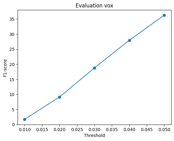
Weighting the positive class recovers non-empty surfaces, but the predictions are over-inflated, smooth volumes that extend beyond the chair and lack its structure. With only one feature vector per image and a small MLP, the network mostly learns a coarse “where is the object” field, and the high positive weight biases it toward over-filling. It stays below the explicit voxel decoder (41.58).
3.2 Parametric Network
The parametric decoder represents the surface as 10 patches, in the style of AtlasNet. Patch
k is an MLP that maps a 2D sample (u, v) ∈ [0, 1]², together with the image feature, to a
3D point: Linear(512+2→256) → ReLU → Linear(256→128) → ReLU →
Linear(128→3), with separate weights per patch (1.65 M parameters in total, against 3.60 M for
the plain point decoder). During training, each patch receives 100 freshly drawn random (u, v) samples
per step. At evaluation, it receives a fixed 10×10 (u, v) grid, which makes the output deterministic
and lets each patch be triangulated into a surface. The model is trained with the same chamfer loss and
settings as 2.2 (1,000 points, batch size 8, lr 4e-4, 2,000 iterations), via
train_model.py --type point --parametric.
F1@0.05 = 68.14


| Decoder | F1@0.01 | F1@0.02 | F1@0.03 | F1@0.04 | F1@0.05 |
|---|---|---|---|---|---|
| Free points (2.2) | 3.50 | 17.84 | 39.44 | 59.39 | 73.31 |
| Parametric, 10 patches | 3.98 | 20.34 | 40.34 | 56.49 | 68.14 |
Tighter but less complete. At the main threshold, the parametric decoder is 5.17 F1 below the free point decoder (paired 95% CI 4.47 to 5.86) and better on only 20% of the test chairs. At the strict thresholds (0.01–0.03), however, it is slightly ahead. Points that lie on smooth sheets sit closer to a surface than the fuzzy cloud of 2.2 does, so more of them pass a tight threshold. However, ten flat-ish sheets cannot cover every leg and armrest, so at looser thresholds the missing coverage (recall) dominates. Per-chair scores of the two models are strongly correlated (r = 0.86), so the hard chairs from 2.5 remain hard.
What the patches learned. I measured the shape of each patch by the ratio of the second to the first singular value of its points (1 = a square sheet, 0 = a line). Averaged over 97 test chairs, 7 of the 10 patches form proper 2D sheets, but 3 have a ratio of 0.21 or less: they have collapsed into thin strips (the red, purple and pink patches in the figure). A strip can still cover a chair leg, so chamfer loss gives no reason to spread it out. Each patch also keeps the same job across chairs: a patch's centre moves by only 0.03–0.07 between chairs, while different patches are about 0.11 apart. In the examples above, the grey patch forms the back of every chair. This is a coarse, consistent part decomposition that the network found without any part labels.
What it offers. The output is a set of surfaces rather than loose points. It can be triangulated directly (third column above), and because (u, v) is continuous, the model can produce any number of points at test time without retraining.