Assginment 2: Single View to 3D
1. Exploring loss functions (10 points)
1.1. Fitting a voxel grid (4 points)

1.2. Fitting a point cloud (3 points)
1.3. Fitting a mesh (3 points)
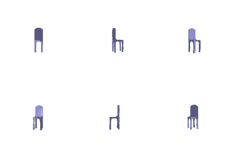

2. Reconstructing 3D from single view (80 points)
2.1. Image to voxel grid (20 points)
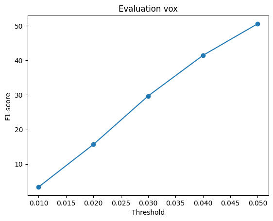
Avg F1@0.05: 48.719
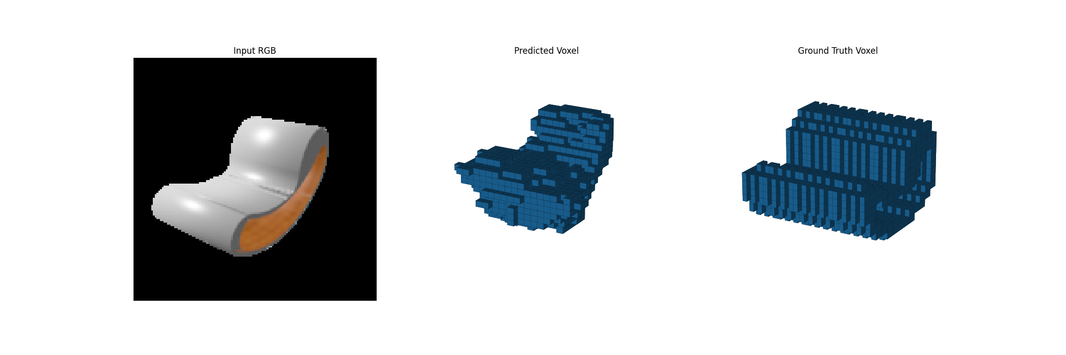
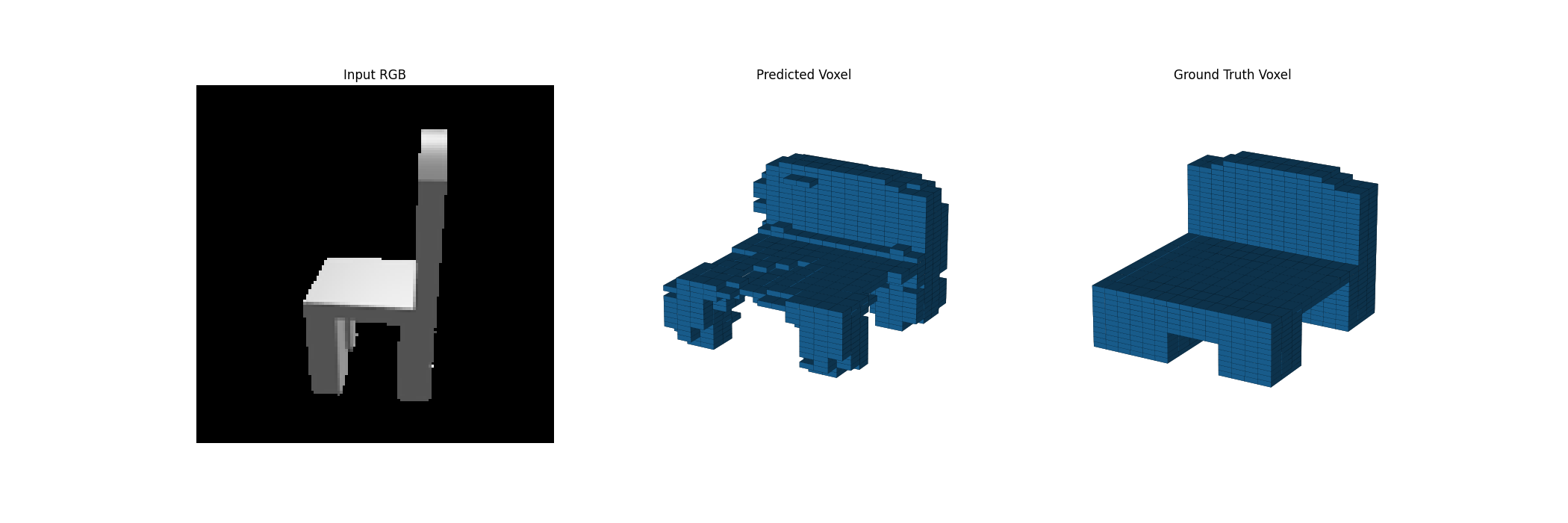
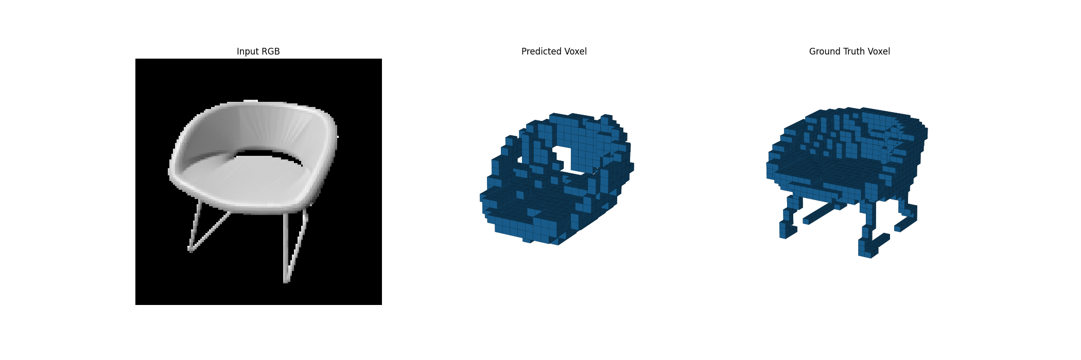
F1 Plot:
2.2. Image to point cloud (20 points)
Avg F1@0.05: 73.023
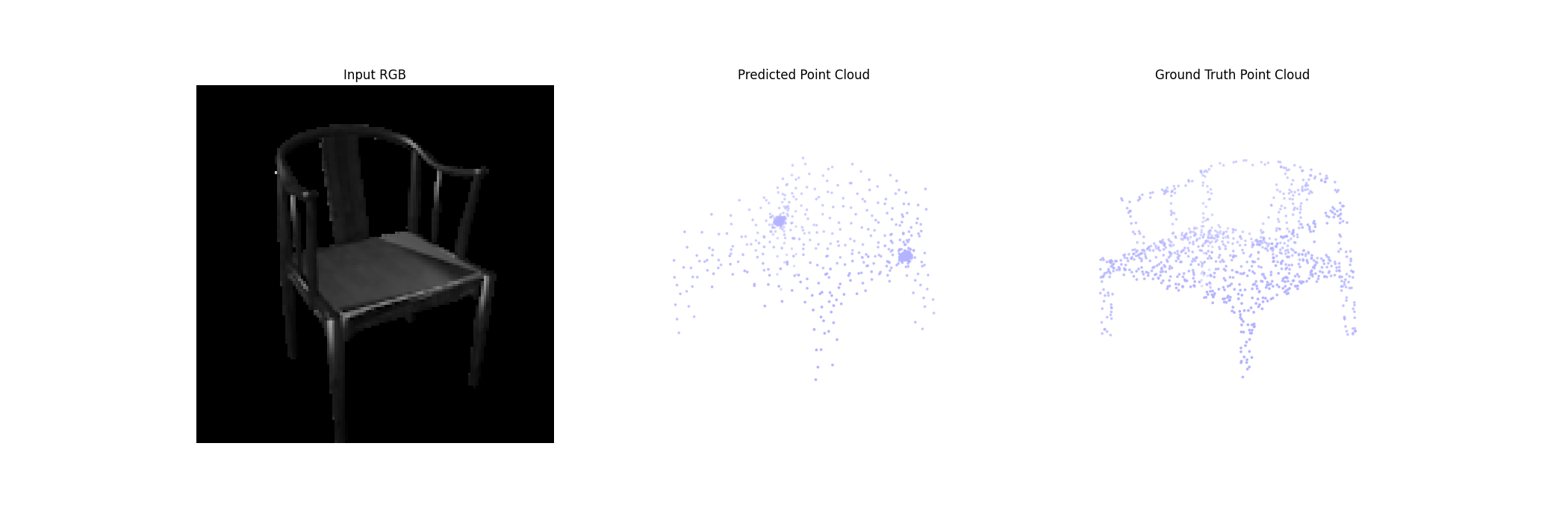
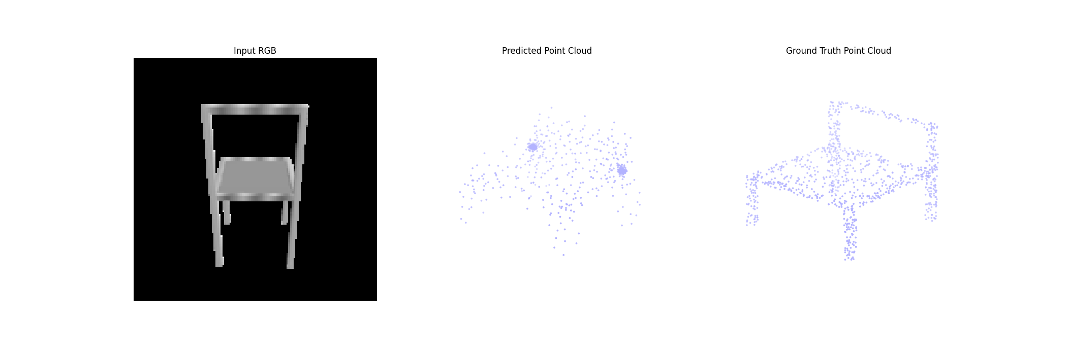
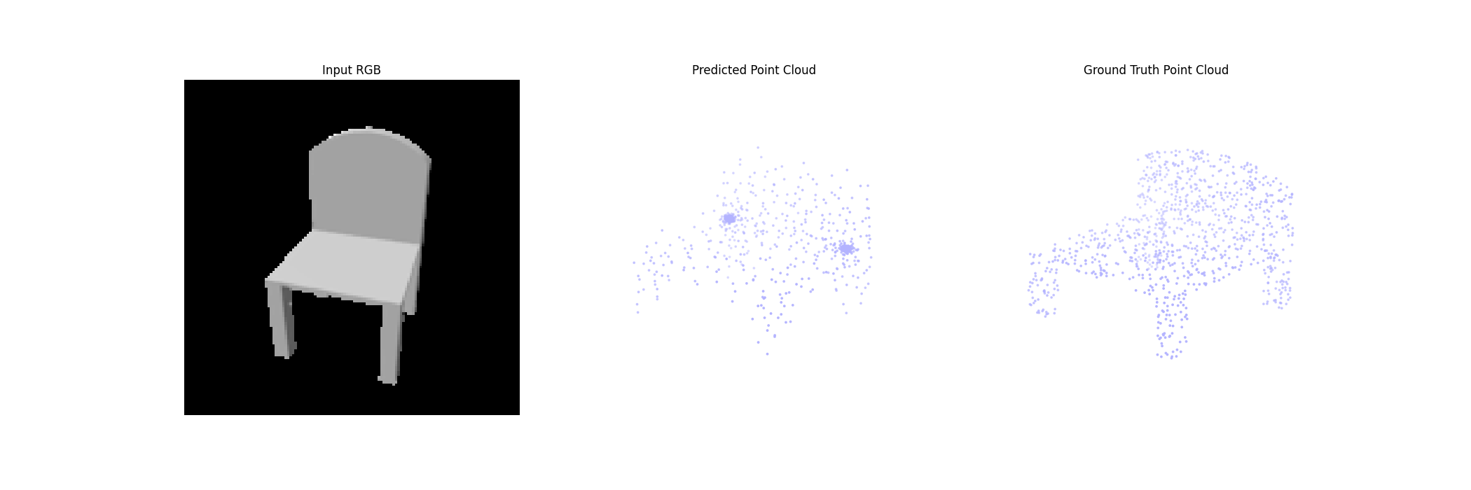
F1 Plot:
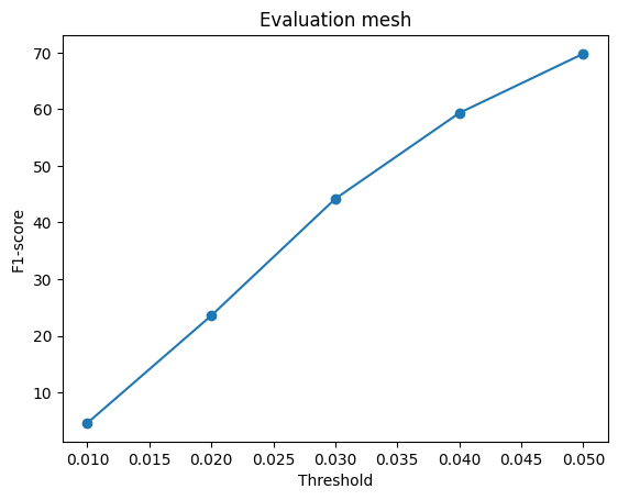
2.3. Image to mesh (20 points)
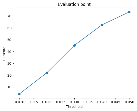
Avg F1@0.05: 69.329
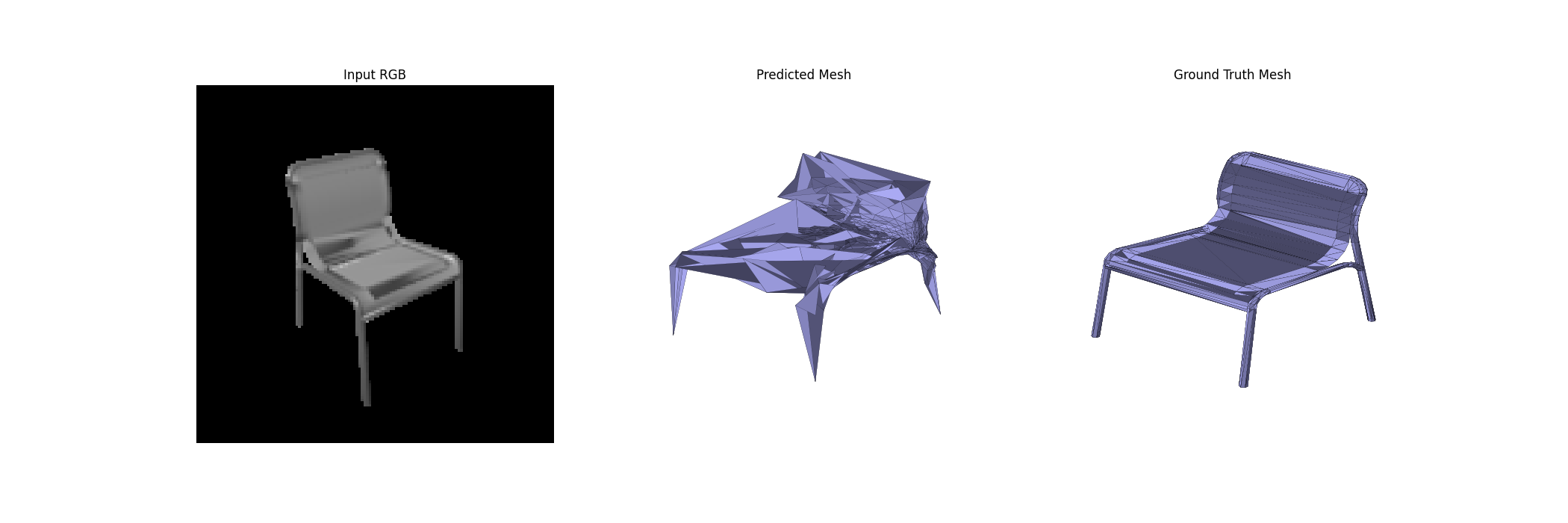
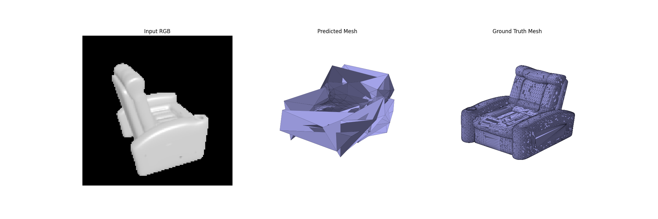
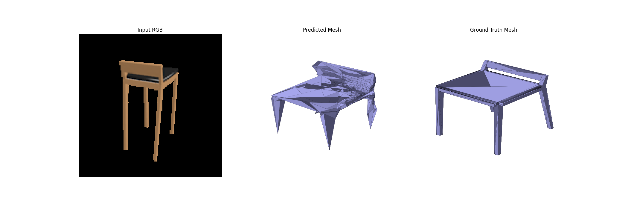
F1 Plot:
2.4. Analyse effects of hyperparams variations (10 points)
I experimented the effect of relative weighting of the directions in the Chamfer distance, and see how the parameter affects the point cloud reconstruction.
I add a weighting parameter alpha, and change the Chanfer distance to: loss_chamfer = (loss_src * alpha + loss_tgt * (1.0-alpha)) * 2
I mulitple the loss with 2 to evaluate with the original loss: loss_chamfer = loss_src + loss_tgt
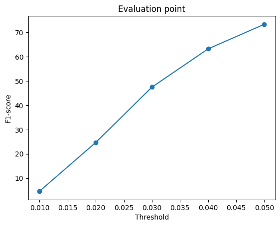
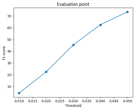
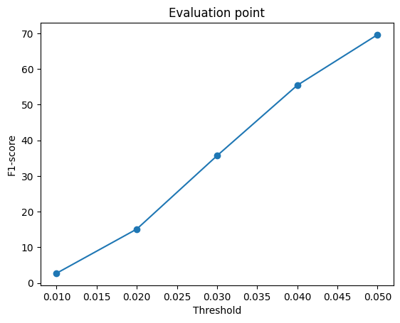
I compare the original one with additional two alpha values: 0.25, 0.75
The result:
| alpha | Precision@0.05 | Recall@0.05 | F1@0.05 |
|---|---|---|---|
| 0.25 | 66.924 | 80.955 | 72.740 |
| 0.50 | 74.794 | 73.442 | 73.023 |
| 0.75 | 82.435 | 63.978 | 70.023 |
The result shows that when alpha increases from 0.25 to 0.75, the precision increases from 66.924 to 82.435. Increase alpha means that we emphasize the predict to ground truth direction, but the trade-off is the recall decrease. Therefore, the F1@0.05 with alpha=0.75 even lower than the value with alpha=0.25.
I also plot the F1 Plot for each alpha value:
2.5. Interpret your model (10 points)
To intepret the effect of chamfer weighting in experiment 2.4, I visualized two distance, Pred to GT distance and GT to Pred distance, in heatmap.
alpha=0.25:
The GT->Pred Distance graph shows more blue points which means that model covers the ground truth shape more completely, so the error of GT to Pred is smaller. And Pred->GT error is larger, many red points distribute over the graph.

alpha=0.5:
This model shows the balance between alpha=0.25 and alpha=0.75, more points focus on the accurate area than alpha=0.25, which also means that the points not coverage as much as alpha=0.25.

alpha=0.75:
The point cloud focus on several accurate areas, so many ground truth shape is not covered. In the GT->Pred Distance graph, you can see the heatmap has a log of red points, and the recall value is lowest.

3. Exploring other architectures / datasets. (Choose at least one! More than one is extra credit)
3.3 Extended dataset for training (10 points)
I choose point cloud to train and evaluate. Compare the quantitative and qualitative results of "training on one class" VS "training on three classes"
Result:
| Training Set | Precision@0.05 | Recall@0.05 | F1@0.05 |
|---|---|---|---|
| Chair only | 74.794 | 73.442 | 73.023 |
| Chair, car, and plane | 77.833 | 77.201 | 76.223 |
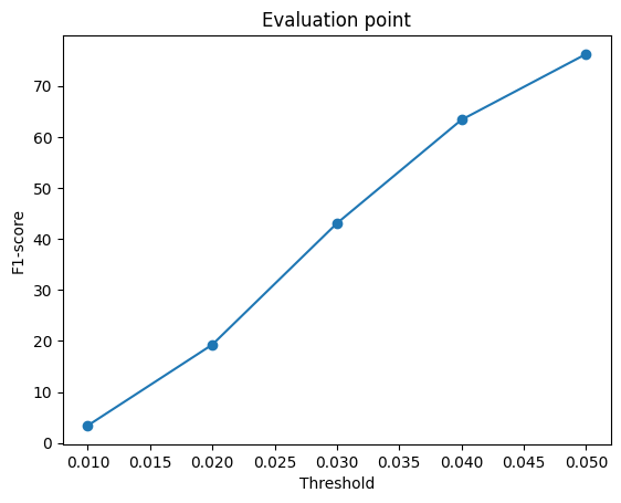
The result shows that training on the extended dataset improved chair reconstruction. The value of F1 increases from 73.023 to 76.223, and in the chart, you can see Precision@0.05 and Recall@0.05 both increase. The quantitative accurancy improved with extended model, but the output diversity seems similar with the chair-only model.
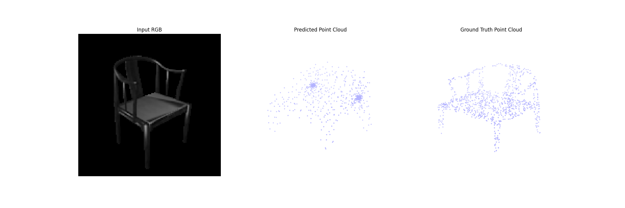
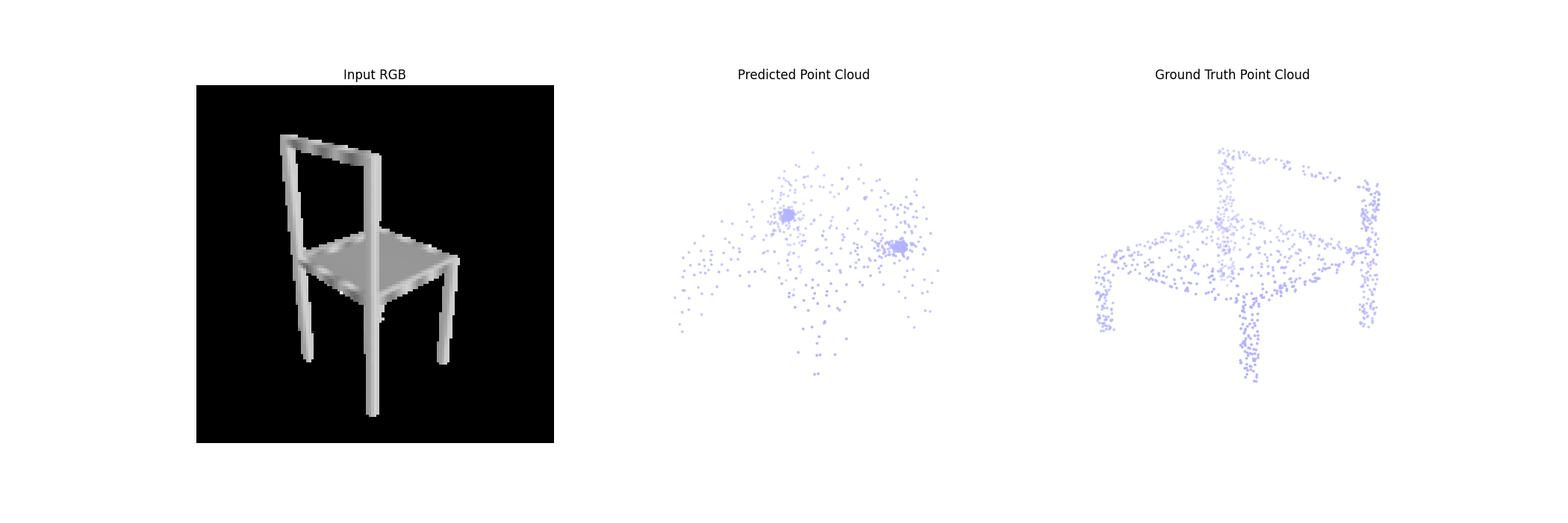
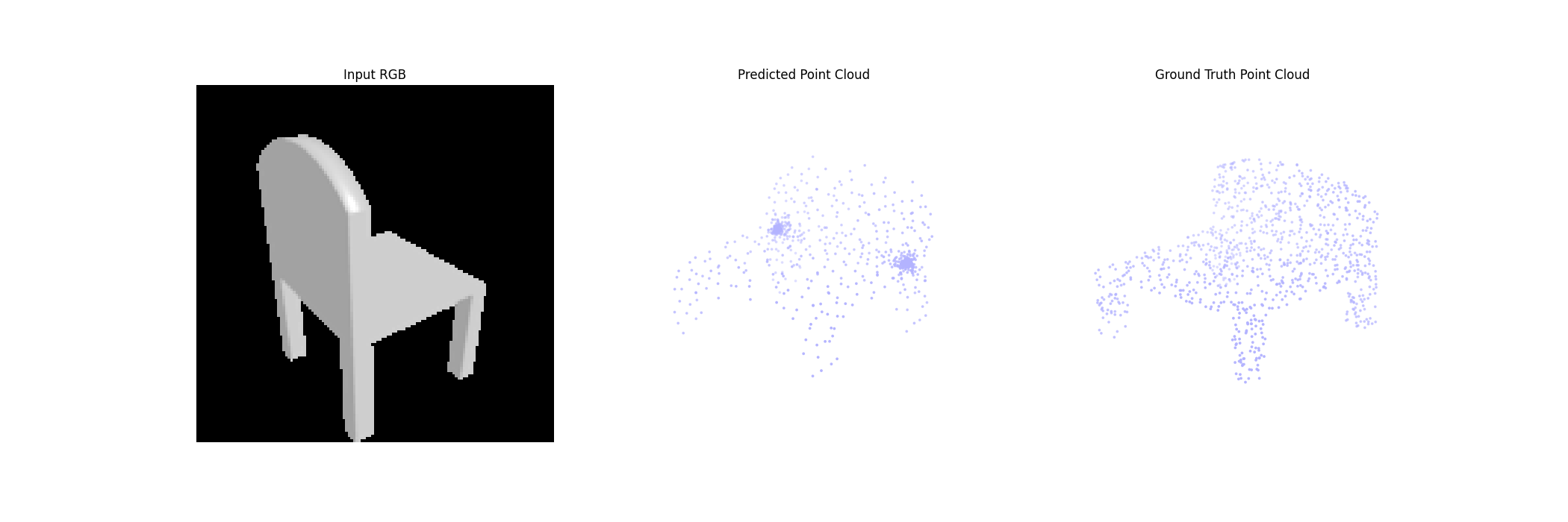
F1 Plot: