16-825 Assignment 2: Single View to 3D
--load_feat option
(precomputed features) was not used.
1. Exploring loss functions
1.1 Fitting a voxel grid
Optimized for 3000 iterations with Adam (lr 4e-4) from a random initialization. The fitted grid is converted to a mesh by marching cubes at probability 0.5 for rendering.

1.2 Fitting a point cloud
Optimized for 3000 iterations (Adam, lr 4e-4) on 5000 points initialized from a Gaussian.

1.3 Fitting a mesh
Optimized for 5000 iterations (Adam, lr 4e-4).

2. Reconstructing 3D from a single view
2.1 Image to voxel grid
Training: batch 128, Adam lr 1e-3, 3000 steps. Training the model for 3000 more steps could have give better F1 score
F1@0.05 = 58.7
| Threshold | 0.01 | 0.02 | 0.03 | 0.04 | 0.05 |
|---|---|---|---|---|---|
| F1 | 4.0 | 18.9 | 35.9 | 49.2 | 58.7 |


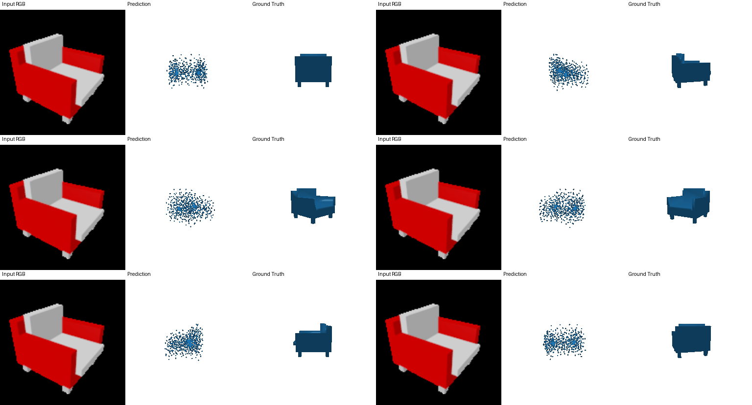
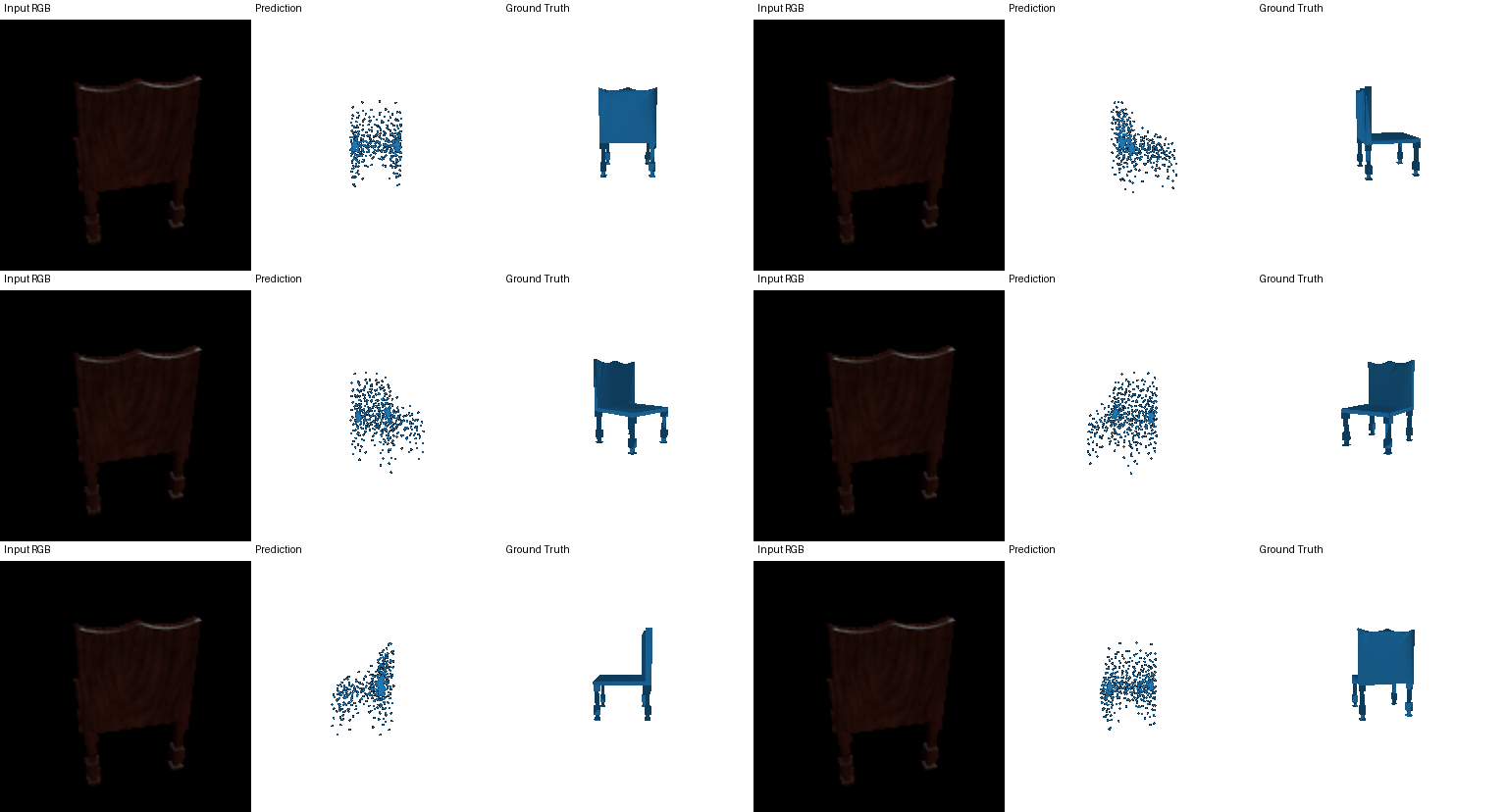
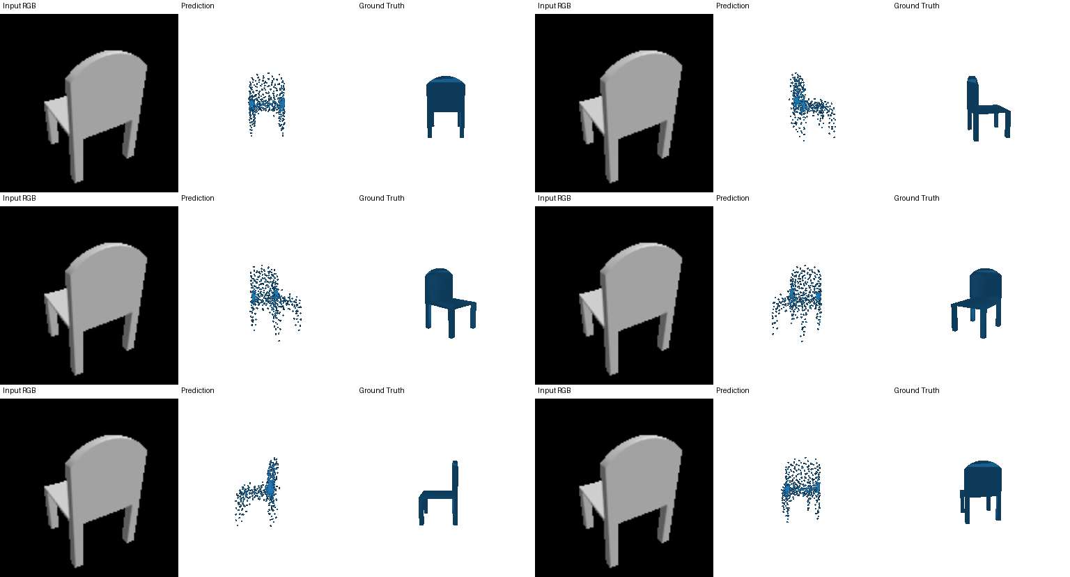
2.2 Image to point cloud
Training: batch 32, Adam lr 4e-4, 6000 steps.
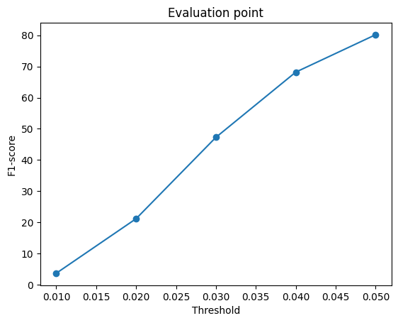
F1@0.05 = 80.2
| Threshold | 0.01 | 0.02 | 0.03 | 0.04 | 0.05 |
|---|---|---|---|---|---|
| F1 | 3.6 | 21.2 | 47.4 | 68.1 | 80.2 |
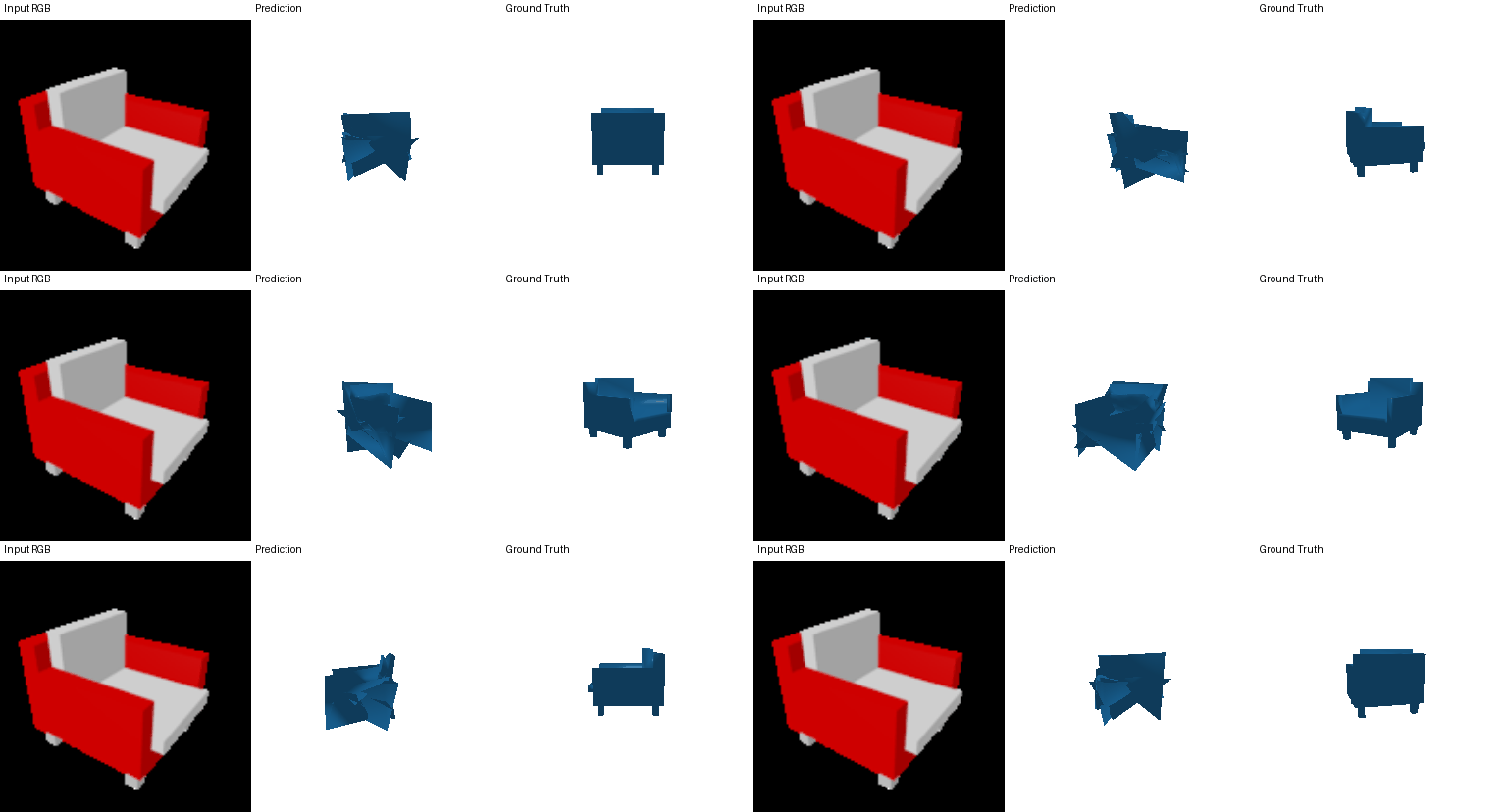
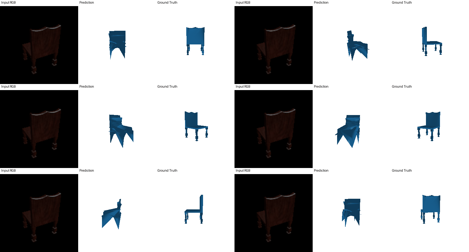
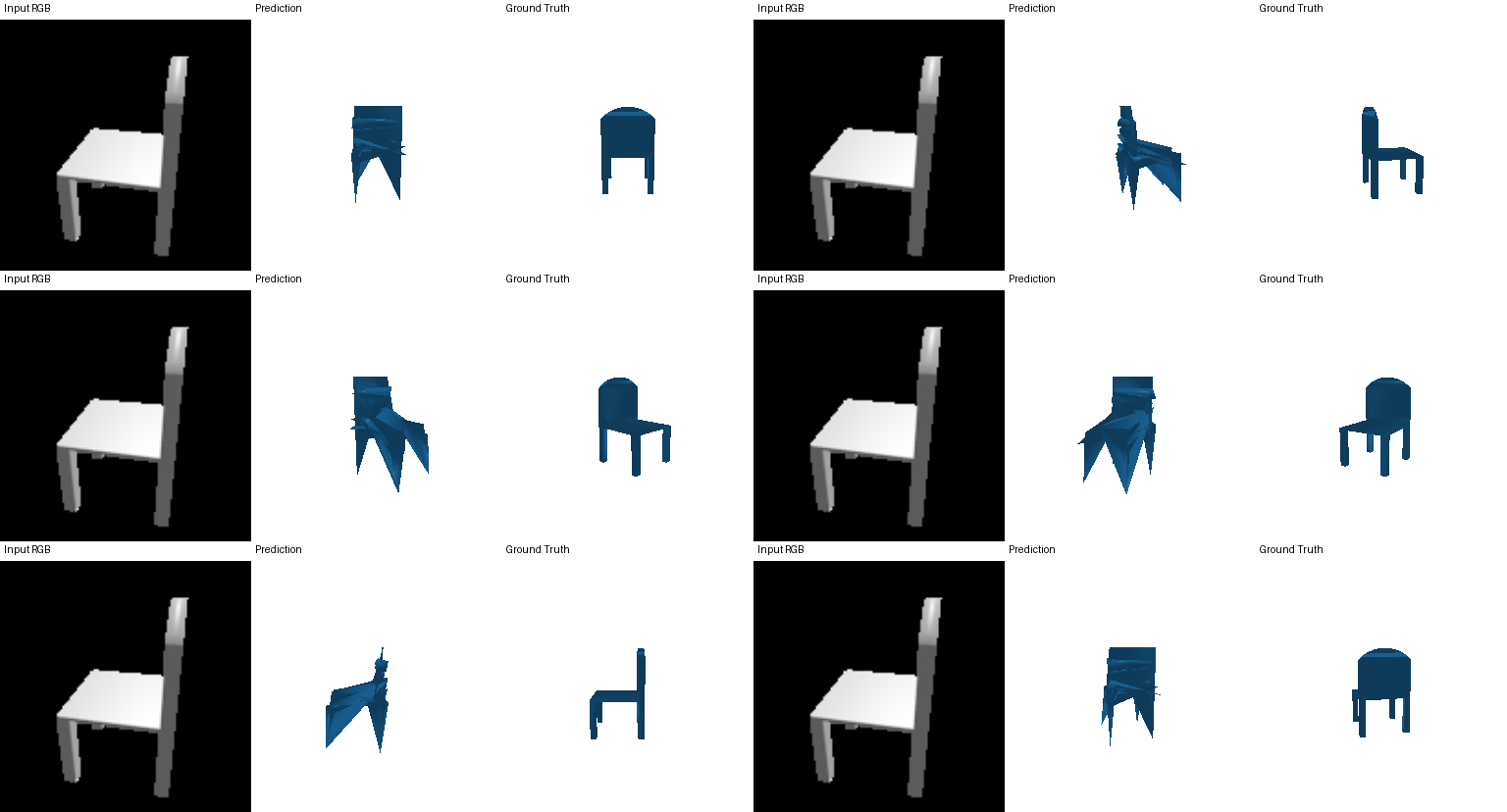
2.3 Image to mesh
Training: batch 32, Adam lr 4e-4, 6000 steps.
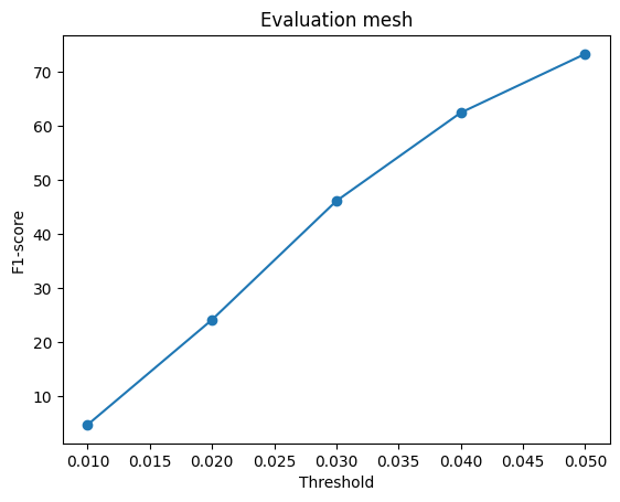
F1@0.05 = 73.3
| Threshold | 0.01 | 0.02 | 0.03 | 0.04 | 0.05 |
|---|---|---|---|---|---|
| F1 | 4.7 | 24.1 | 46.1 | 62.5 | 73.3 |
Comparing voxels, point clouds and meshes
| Representation | F1@0.01 | F1@0.02 | F1@0.03 | F1@0.04 | F1@0.05 |
|---|---|---|---|---|---|
| Point cloud | 3.6 | 21.2 | 47.4 | 68.1 | 80.2 |
| Mesh | 4.7 | 24.1 | 46.1 | 62.5 | 73.3 |
| Voxel grid | 4.0 | 18.9 | 35.9 | 49.2 | 58.7 |
Point cloud > mesh > voxel grid.
- Point clouds are trained with chamfer distance, which is something that F1 loss also optmizes for. Every point is free to move independently, with no connectivity to respect, so the network can place points exactly where the surface is, including on thin legs.
- Meshes are also trained with chamfer, but they can't represent genus-0 topology. A chair with holes between its legs and backrest cannot be represented exactly, so thin parts are rounded off and gaps get bridged by stretched faces.
- Voxels are limited by resolution: at 32³ a chair leg is about one voxel wide, so whether it survives depends on a single cell crossing the 0.5 threshold.
2.4 Effect of the Laplacian smoothness weight (w_smooth)
I trained the image-to-mesh model twice with identical settings, changing only the smoothness weight: the default
w_smooth = 0.1 and a 10× larger w_smooth = 1.0.
w_smooth | F1@0.01 | F1@0.02 | F1@0.03 | F1@0.04 | F1@0.05 |
|---|---|---|---|---|---|
| 0.1 | 4.651 | 23.853 | 45.543 | 61.932 | 73.080 |
| 1.0 | 4.422 | 22.465 | 42.510 | 57.608 | 68.340 |
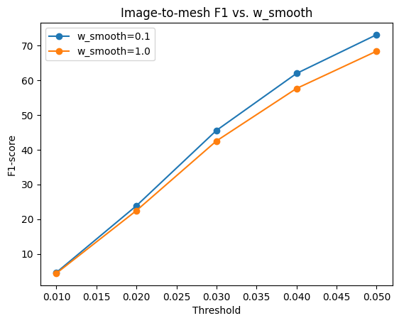
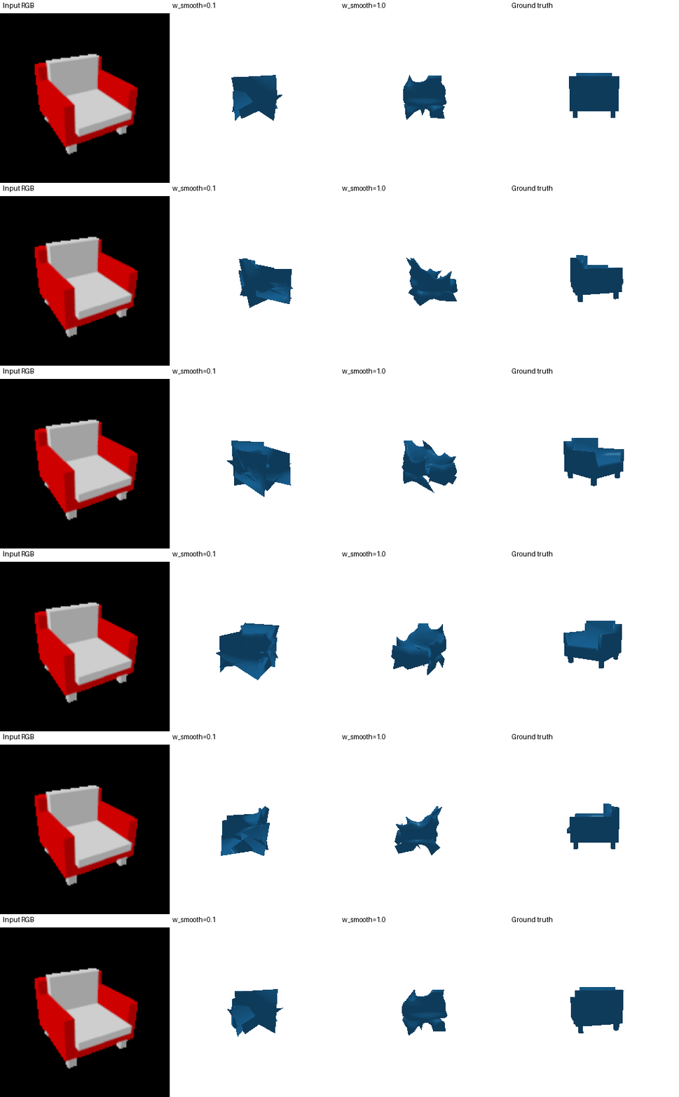
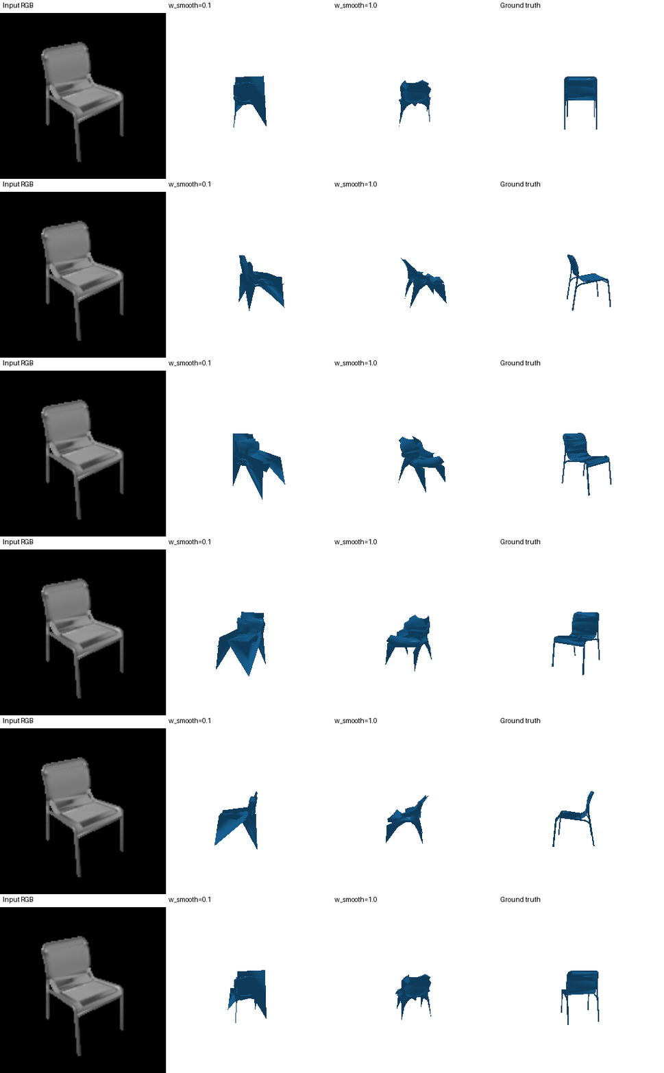
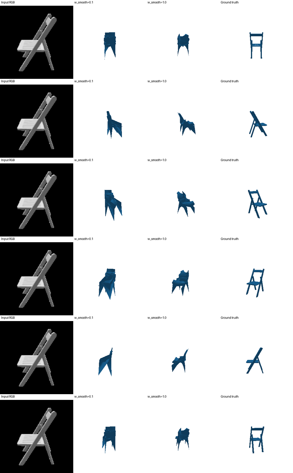
Analysis. Increasing w_smooth from 0.1 to 1.0 makes the meshes
visibly cleaner, fewer spikes, and more rounded
blob-like surfaces. But F1 is lower.
The Laplacian term pulls each vertex toward the average of its neighbors, which directly fights
the sharp, thin geometry that chairs are made of, legs get shortened and armrests and seat edges
pulled inward. The conclusion is that smoothness is a trade-off: a small weight might give visually worse artifacts, while a large
weight gives visual tidiness at the cost of geometric accuracy.
2.5 Interpreting the model: where do the points go wrong?
F1 compresses two different failure modes into one number- predicted points that are in the wrong place (precision) and parts of the object that nothing covers (recall). To see both, I colored every point by the same distance test the metric uses (τ = 0.05), for the point-cloud model from 2.2:
- Predicted points, by distance to the nearest ground-truth point: green = correct (< 0.05), orange = near miss (0.05–0.1), red = extra / hallucinated (≥ 0.1).
- Ground-truth points, by distance to the nearest predicted point: gray = covered, purple = missing (no prediction within 0.05).
The green fraction is the precision and the gray fraction is the recall, so each GIF shows which parts of the chair the score is lost on.


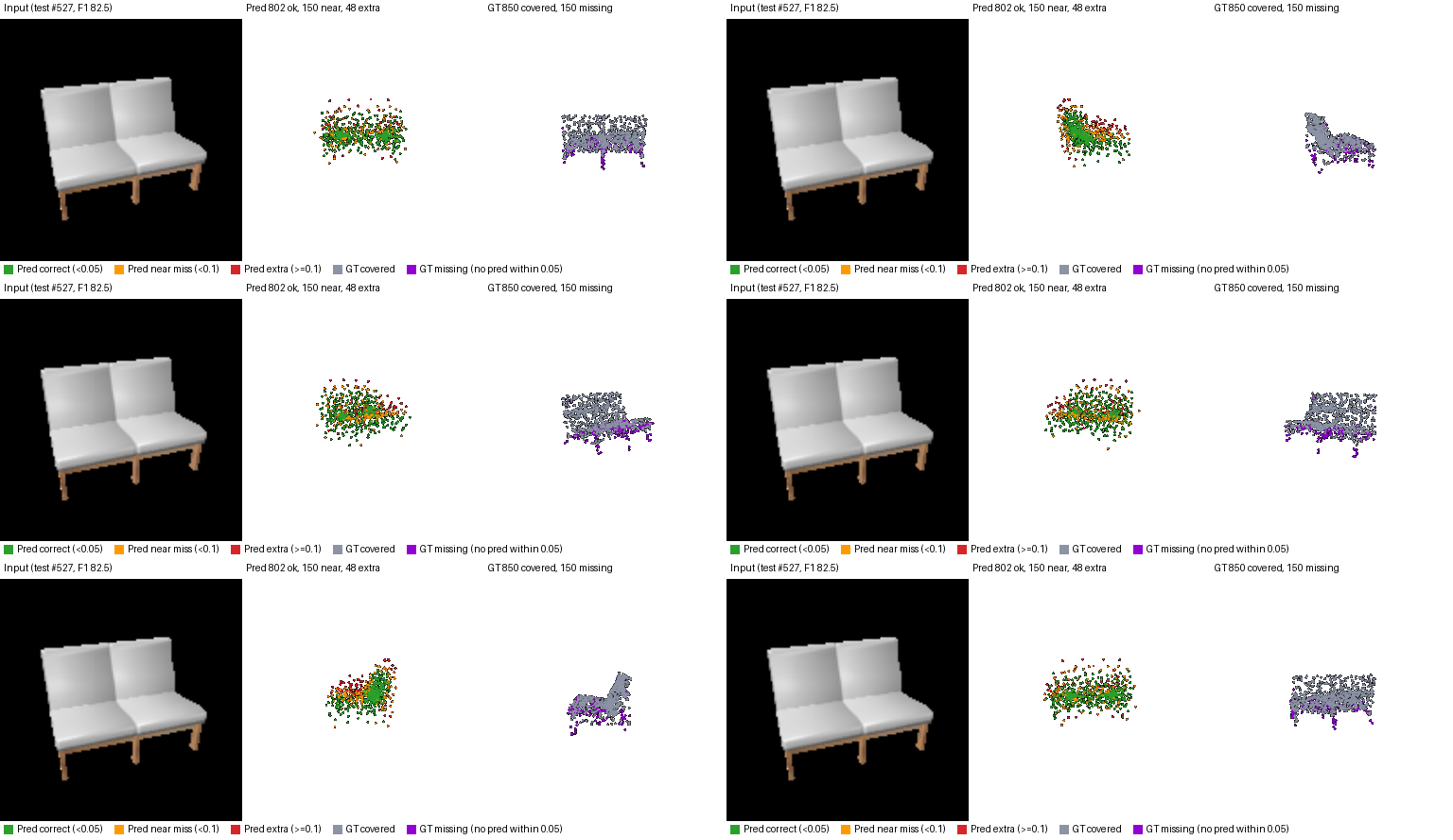
Analysis: The model reliably reconstructs the bulky central mass of a chair (seat, cushions), where almost all predictions are green and almost all ground truth is gray.Recall is lost on thin, far-from-center structures: legs, backrests and armrest edges are purple. Precision is lost as a halo of orange and red points around the outline, where the model is indecisive between plausible positions instead of committing to one. Chairs with more thin structure (test #150) score noticeably lower than bulky ones (test #301), even though the overall shape is right in both.
3. Exploring other architectures and datasets
3.1 Implicit network
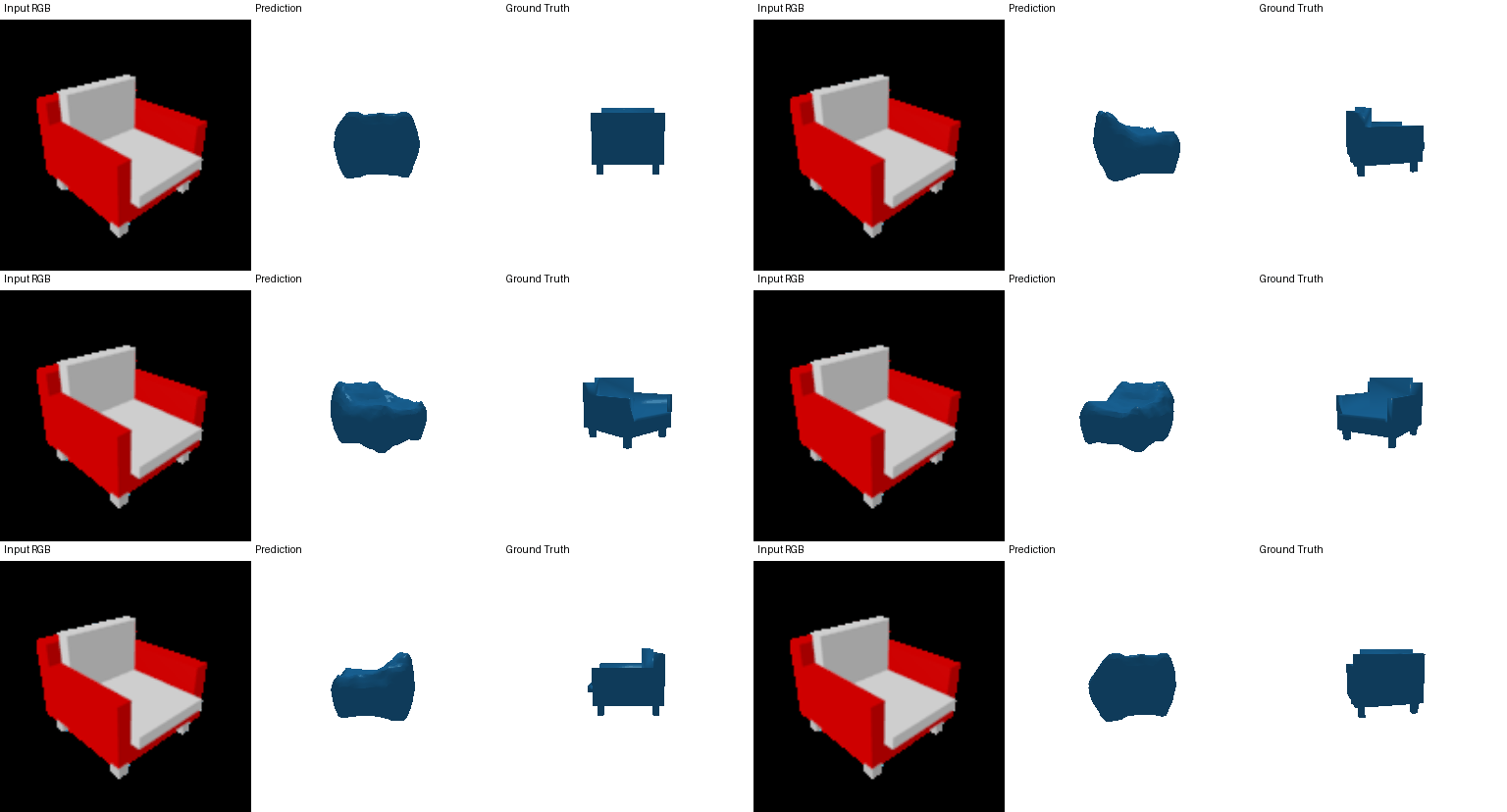
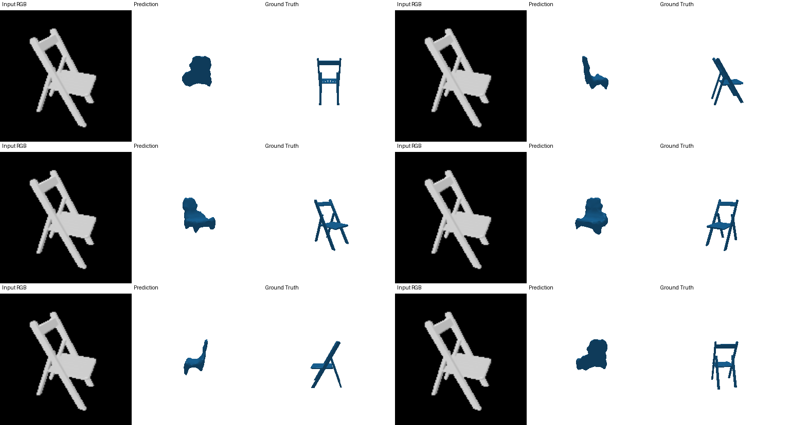
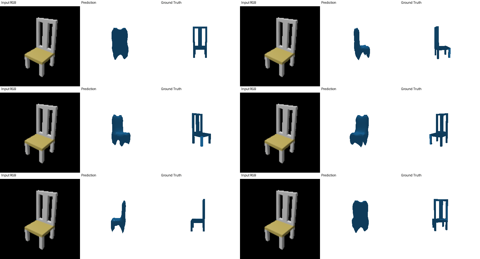
Architecture: The query point x ∈ (-1,1)³ is encoded with Sin/Cos positional encoding and combined with the 512-d ResNet18 image feature in a linear layer to 256 units, followed by three residual blocks (256→256, ReLU) and a linear output. At test time the network is queried on the full 32×32×32 meshgrid of (-1,1)³, and the resulting occupancy grid is converted to a mesh with marching cubes and evaluated exactly like the voxel model.
Training: binary cross-entropy against the ground-truth voxels on
all 32³ grid cells each step, with occupied cells weighted 3×
(pos_weight = 3); batch 32, Adam lr 2e-4; 3000 steps.
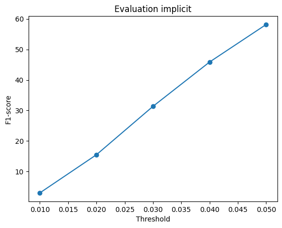
F1@0.05 = 58.140
| Implicit model | F1@0.01 | F1@0.02 | F1@0.03 | F1@0.04 | F1@0.05 |
|---|---|---|---|---|---|
Final: all cells, pos_weight 3 | 3.023 | 15.510 | 31.352 | 45.858 | 58.140 |
3.2 Parametric network
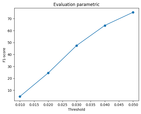
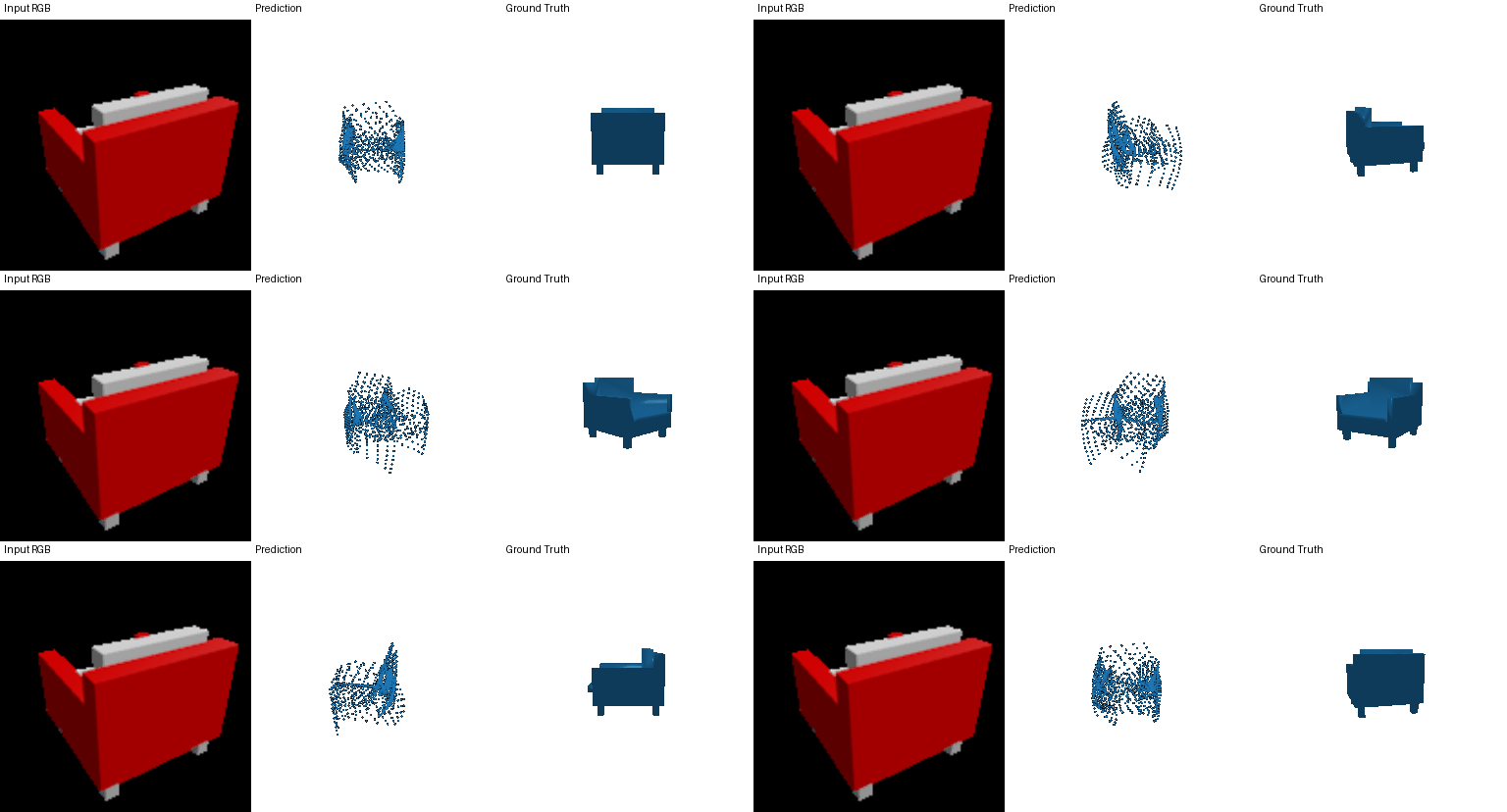
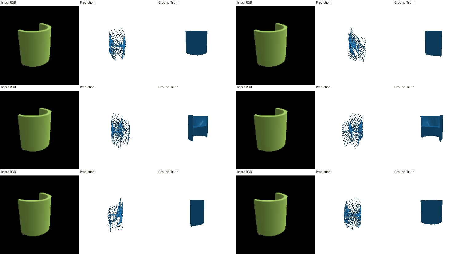
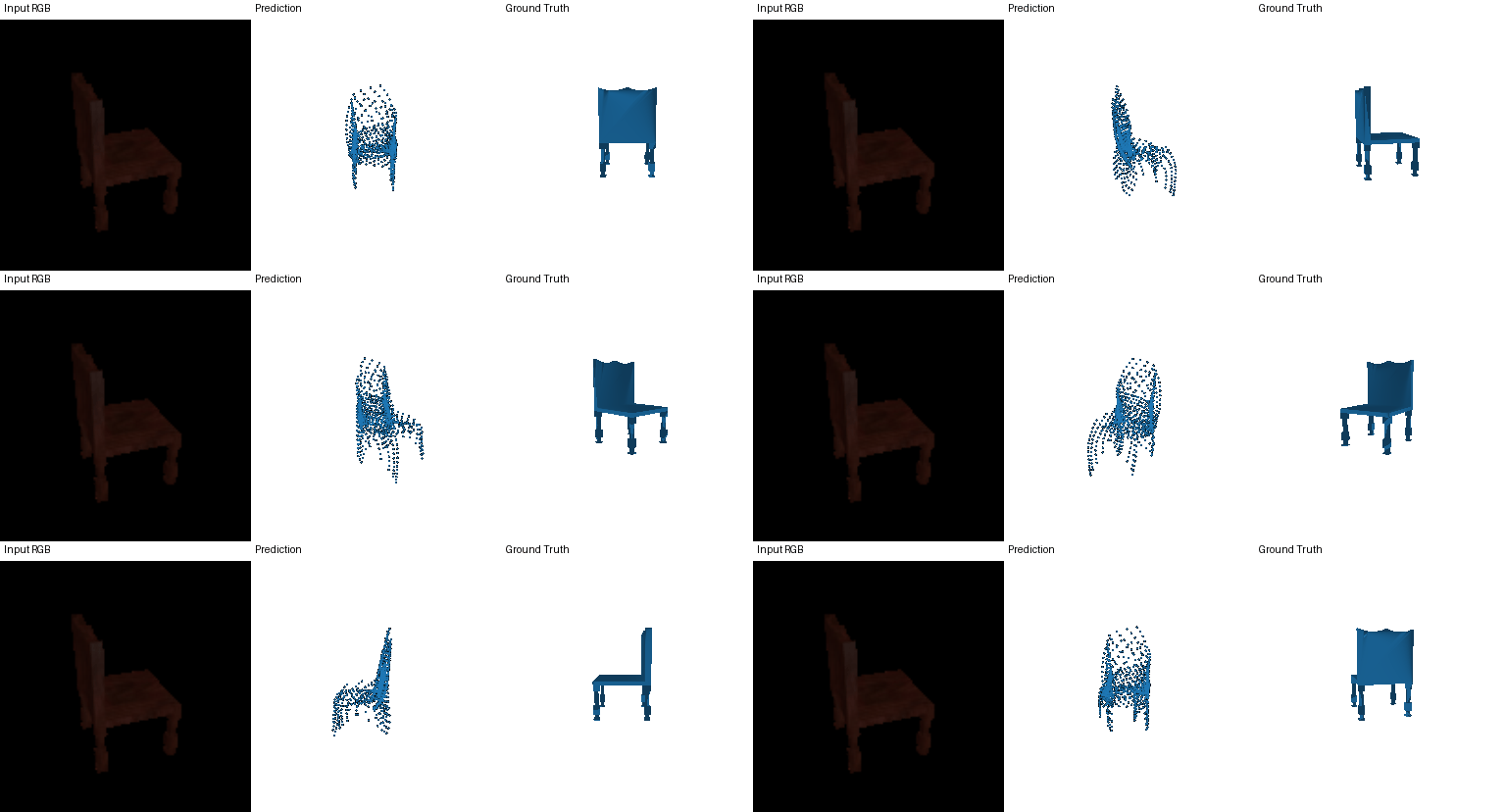
Architecture (AtlasNet-style): 4 surface patches, each a small MLP (514 → 256 → 256 → 128 → 3, ReLU) that maps a 2D sample (u, v) ∈ [0,1]², concatenated with the 512-d image feature, to a 3D point. Each patch learns one parametric piece of the surface, and their union covers the object.
Training: every step samples fresh random (u, v) points (250 per patch, 1000 in total) and minimizes chamfer distance to 1000 points sampled from the ground-truth mesh; batch 32, Adam lr 4e-4, 3000 steps. A
F1@0.05 = 75.321
| Threshold | 0.01 | 0.02 | 0.03 | 0.04 | 0.05 |
|---|---|---|---|---|---|
| F1 | 4.845 | 24.525 | 47.417 | 64.291 | 75.321 |
With only 3000 training steps the parametric network comes close to the point-cloud decoder from 2.2, which trained for 6000 steps.
3.3 Training on an extended dataset
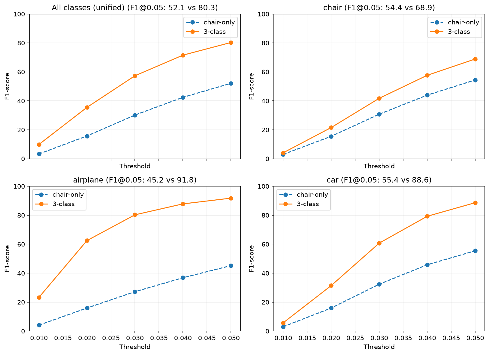
I compared two image-to-mesh models: the chair-only model from 2.3 and the same architecture trained on all three classes (3000 steps). Both are evaluated on the extended dataset's test set with 3 classes
| F1@0.05 / test class | Chair-only model (6k steps) | 3-class model (3k steps) |
|---|---|---|
| Chair | 54.40 | 68.88 |
| Airplane | 45.19 | 91.78 |
| Car | 55.43 | 88.64 |
Note: the two models were not trained for the same number of steps because of limited compute resources. The chair-only model was trained for 6k steps and the 3-class model for only 3k steps, so the comparison is not step-matched, and the size of the gap should be read with that in mind. The 3-class model scores higher on every class despite having half the training.
Each GIF shows Input RGB | chair-only model | 3-class model | Ground truth:


Analysis.
- The chair-only model forces every input into a chair. Given an airplane or a car, it still outputs a tall, chair-like structure, because it has only ever learned to deform the sphere into chairs. Its F1 score on airplanes and cars is also poor.
- Diversity vs. consistency. The chair-only model's outputs collapse onto one class prior regardless of the image. The 3-class model's outputs are much more diverse.
- Airplanes and cars are easier than chairs. Within the 3-class model, airplanes and cars score far above chairs. Chairs have the most thin parts and holes, which a genus-0 mesh cannot represent.