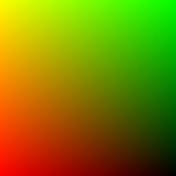
The pixel coordinates cover NDC space from -1 to 1. Each ray starts at the camera center and points through its pixel on the image plane.
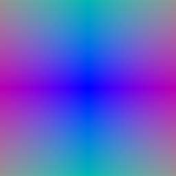
I sampled 64 evenly spaced points from depth 0 to 5 along each ray.
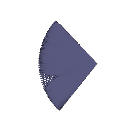
For each sample I computed alpha from density and segment length, multiplied it by the accumulated transmittance, and used the resulting weights to sum color and depth along the ray.
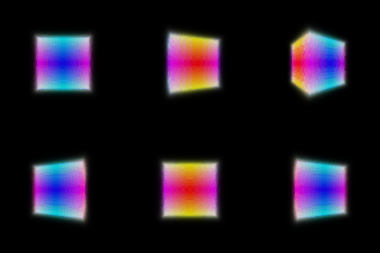
Depth normalized by its maximum value:
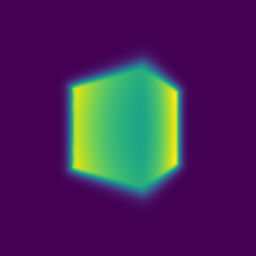
I trained the box for 1000 epochs using 4096 randomly sampled rays per image and RGB mean squared error.
Box center: (0.25, 0.25, 0.00)
Box side lengths: (2.01, 1.50, 1.50)
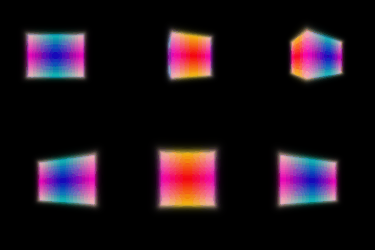
I used six-frequency positional encoding and a six-layer MLP with 128 hidden units and a skip connection at layer 3. I trained for 250 epochs using 1024 randomly sampled rays per image and 128 points per ray.
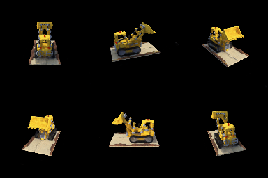
I used the materials scene to compare a position-only NeRF with one that also uses the viewing direction. I embedded the ray direction with two frequencies and fed it into the color layers. Density still only depends on position. Both models were trained for 250 epochs at 128 by 128 resolution with the same settings.
Without view direction:
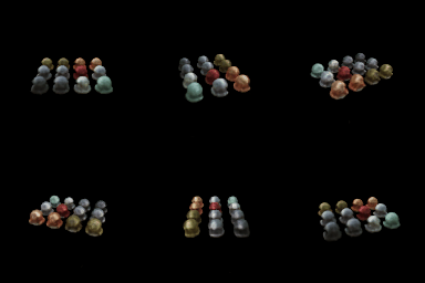
With view direction:
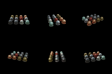
Matching camera views:


Without direction, every point has to use the same color in every view, so the highlights get averaged out. Adding direction gives the metallic objects stronger highlights that move with the camera. The tradeoff is a larger model that can overfit the training camera angles and do worse on very different views.
I first rendered 64 evenly spaced samples with the coarse network. I used its weights to pick 64 more samples around the occupied parts of the ray, combined and sorted all the samples, and rendered them with a separate fine network. I trained both outputs with RGB mean squared error for 250 epochs.
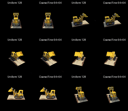
On ten held-out views the fine result was much better than its 64-sample coarse result. It was still a little worse and slower than the Part 3 model, even though both used 128 samples per ray in total:
| Method | PSNR | SSIM | Seconds per image |
|---|---|---|---|
| Coarse, 64 uniform samples | 11.595 | 0.572 | 0.050 |
| Coarse/fine, 64+64 samples | 23.585 | 0.877 | 0.145 |
| Part 3, 128 uniform samples | 24.741 | 0.896 | 0.110 |
The fine pass helped because it spent more samples around the bulldozer instead of empty space. However, it also had to run a second network, and the 64-sample coarse result was not accurate enough to beat the simpler 128-sample model. More coarse or fine samples would probably help quality, but would make rendering even slower.
I projected the 3D Gaussians onto the image, sorted them by depth, and discarded the ones behind the camera. At each pixel I blended color, depth, and silhouette from front to back using alpha and transmittance.
The animation shows the RGB render, colored depth, and silhouette mask for each view.
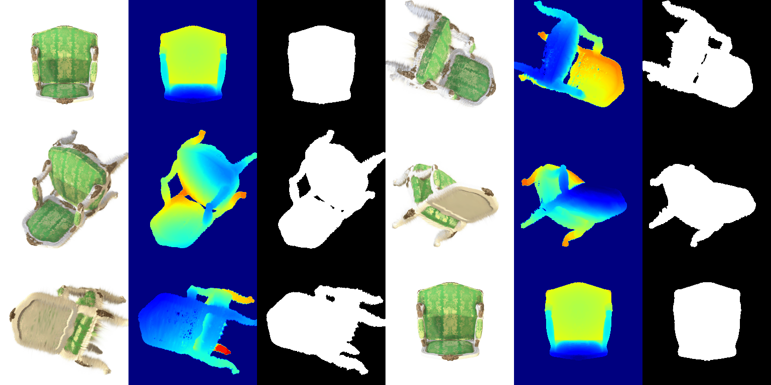
I trained 10,000 isotropic Gaussians for 1,000 iterations with RGB L1 loss. I used learning rates of 0.05 for opacity, 0.005 for scale, 0.01 for color, and 0.0001 for position. I did not optimize quaternion rotations because the Gaussians were isotropic.
Held-out PSNR: 29.294
Held-out SSIM: 0.938
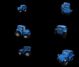
Training progress, with predictions on top and ground truth on the bottom:
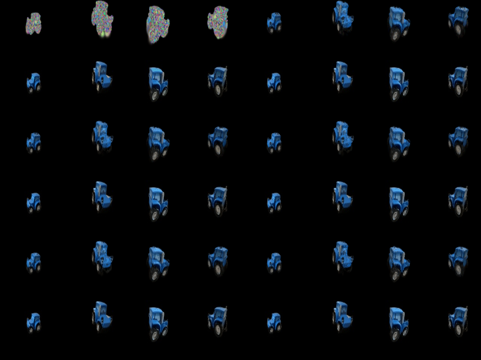
Final training-view renders:
The file has 16 spherical harmonic coefficients for each color channel. I evaluated them using the direction from the camera to each Gaussian. The original render only uses a constant color.
Without spherical harmonics:
With spherical harmonics:

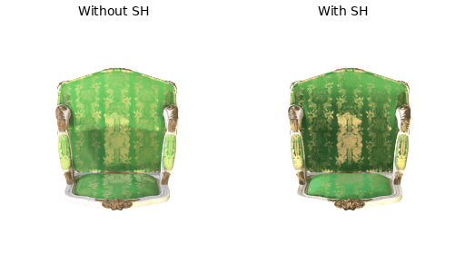
This is a front view. With SH, the chair back is darker and the gold pattern stands out more. The shape stays the same.
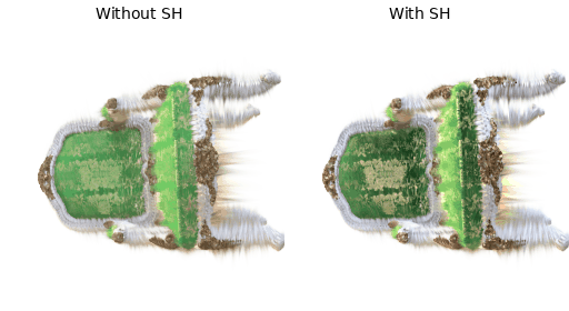
This view is almost from the top and side. With SH, the green fabric is darker and the pattern is easier to see. The long fuzzy splats around the edges are in both versions because SH only changes color.
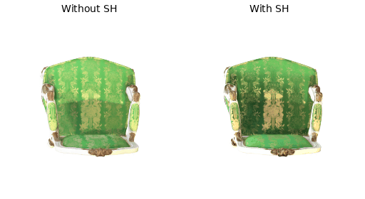
This is another front view. With SH, the back and wooden trim are darker and the pattern has more contrast. The silhouette is unchanged.