Andrew ID: mehark
Part A is neural volume rendering (nerf/), part B is 3D Gaussian splatting (GS/). All
PSNRs are means over the 100 held-out views of a scene at 128x128. Everything ran on one
shared A6000 per job.
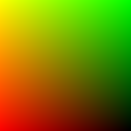
Each pixel is mapped to [-1, 1] in x and y, placed on the image plane at depth 1 and unprojected to world space. A ray then starts at the camera center and poinst through its pixel, with the direction normalized.
xy grid (vis_grid)
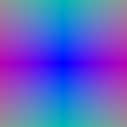
Ray directions (vis_rays)
64 depths evenly spaced between min_depth and max_depth; each sample is
origin + depth x direction.
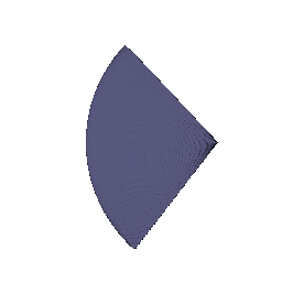
Sample points along the rays of the first camera
For sample i, alpha = 1 − exp(−σΔt) and T is the product of (1 − alpha) over the earlier samples, with T = 1 for the first. The weight is T · alpha. Color is the weighted sum of the sample colors; depth is the weighted sum of the sample depths.
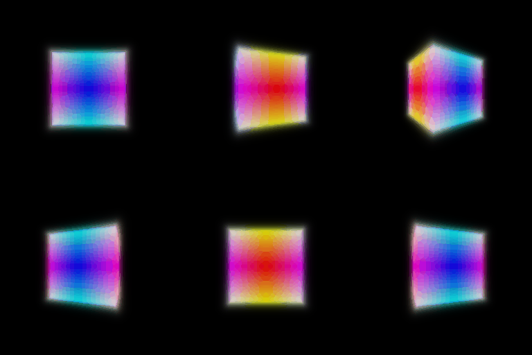
Rendered box (part_1.gif)
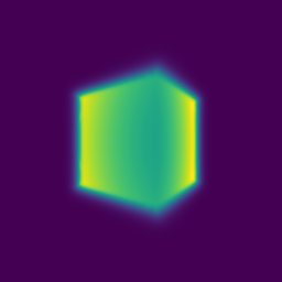
Depth map, normalized by its maximum
2.1: each step uses a random subset of the pixels (shuffle the grid, keep the first N), which keeps the backward pass small. 2.2: the loss is the mean squared error between rendered and ground-truth colors. The box actually converges within the first couple of hundred epochs; the rest of the 1000 only polishes the last digit.
| x | y | z | |
|---|---|---|---|
| Box center | 0.25 | 0.25 | -0.00 |
| Box side lengths | 2.01 | 1.50 | 1.51 |
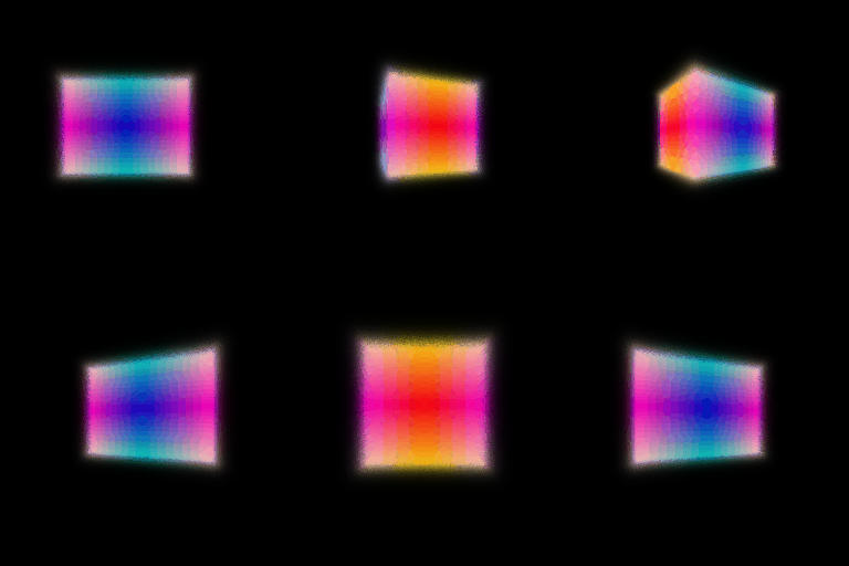
Optimized box (part_2.gif), seemingly identical to the TA reference
Network: the position is positionally encoded with 6 frequencies and goes through a 6-layer MLP of 128 units with ReLU; the encoding is concatenated back in before layer 3 (skip connection). Two heads follow:
Training: MSE loss, 1024 rays per step, 128 samples per ray, 250 epochs on 128x128 lego images.
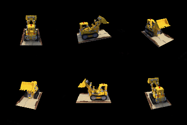
NeRF lego (part_3.gif). Held-out PSNR 24.32 dB.
How: the ray direction is encoded with 2 frequencies and concatenated to the trunk feature just before the color head. Density still depends on position only, so the geometry cannot change with the viewpoint. Trained on the materials scene with and without it, everything else equal.
| Materials, 128x128 | Held-out PSNR |
|---|---|
| no view dependence | 23.35 dB |
| with view dependence | 23.84 dB |

Without view dependence

With view dependence
Trade-off: the materials scene is a grid of shiny spheres, and a position-only color has to paint one average highlight per point, which consequently sits in the wrong place from most views. With the direction in the color head the highlights actually move with the camera (watch the gold and copper spheres in the turntable), and held-out PSNR goes up by half a dB. The gain looks small in PSNR because most pixels are diffuse. The risk runs the other way: the more the network may use the direction, the easier it is to explain every training image with a view-specific color instead of a consistent 3D scene, since from a single camera "this point is bright from here" and "there is a bright surface further alogn the ray" look the same. Three choices keep that in check: density never sees the direction, the direction is encoded with only 2 frequencies so it can only vary smoothly, and it enters late through a small head. Pushing the direction encoding higher sharpens training views and hurts novel ones, substantially so with only 100 training images.
How: two networks with the part 3 architecture. The coarse one is evaluated at 64 evenly spaced samples; its weights, normalized, give a distribution along the ray, and inverse-CDF sampling draws 64 more depths from it, so they land where the coarse pass found content. The fine network is evaluated at all 128 sorted depths and gives the final image. Both networks are trained with MSE.
| Lego, 250 epochs | Samples per ray | Held-out PSNR | Render time per image |
|---|---|---|---|
| single NeRF (part 3) | 128 uniform | 24.32 dB | 0.14 s |
| coarse + fine | 64 + 64 | 24.49 dB | 0.24 s |
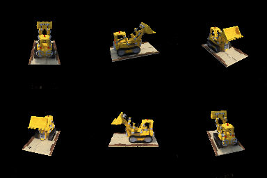
Coarse + fine NeRF (fine network)
Trade-off: the fine pass spends its samples on the surface instead of on the empty space between depth 2 and 6, which is actually where most of the uniform samples go. Quality goes up a little (+0.2 dB, slightly crisper bucket and tracks), and the price is a second network and 192 network evaluations per ray instead of 128, so rendering is about 1.7x slower and training needs more memory. The two trainings ran on different shared GPUs, so the render time measured back to back on one GPU is the number I trust. The benefit would presumably grow with resolution or a larger depth range, since uniform sampling wastes a fixed fraction of its budget on empty space while importance sampling does not.
How:
What α and β do: α is the density deep inside the object, so it sets how opaque a solid is. β is the width of the transition from 0 outside, through α/2 exactly on the surface, to α inside. A small β is a thin, almost hard shell; a large β is fog spread around the surface.
How does high β bias the SDF, and low β? With a high β the density is spread over a thick shell, many samples along a ray contribute, and the surface is only loosely pinned down: the result is smooth and blobby, with thin parts and sharp edges averaged away. With a low β the density sits in a thin shell, so the zero level set actually has to be in the right place and the surface hugs the true shape.
Easier to train with low or high β? High β. The gradient reaches samples far from the current surface, so even a bad initial surface receives a signal and can move. With a low β the loss is almost a step function of the distance, most samples get no gradient, and consequently training stalls unless it starts from a good surface. That is presumably why VolSDF anneals β downwards.
More accurate surface with low or high β? Low β, provided it trains. The rendered color then depends on a thin layer at the zero crossing, so the SDF must put that crossing on the object and the extracted mesh is crisp. With a high β the image can look fine while the surface is off.
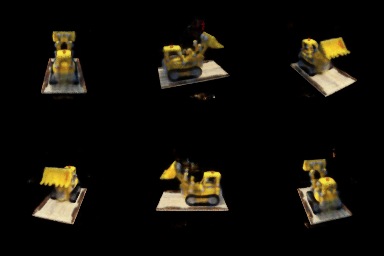
VolSDF color, α = 10, β = 0.05
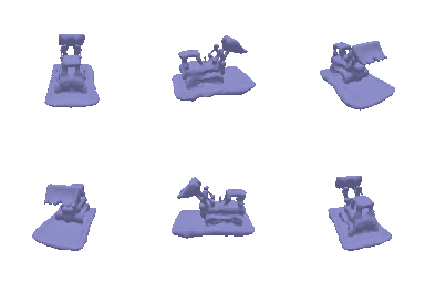
VolSDF geometry (marching cubes of the SDF at 0)
Chosen settings and why: α = 10, β = 0.05, eikonal weight 0.02 and 250 epochs, which are the given config values, plus a sphere initializtaion that actually mattered more than any of them. My first attempt started the distance field "inside everywhere" (a constant negative bias on the output), and with β = 0.05 that is dense fog with no zero crossing anywhere: the color loss was perfectly happy shading the fog, the eikonal term had nothing to pull on, and marching cubes never found a surface. The fix is to have the network predict a residual on top of the signed distance of a sphere of radius 1.5, with the residual initialized near zero. At step 0 the field is exactly a sphere, so the eikonal constraint already holds and there is a real surface for the color loss to push onto the bulldozer. With that in place the given β works as is: the mesh has clean edges and the tracks are separate from the base. A quick try at β = 0.1 trained the same but gave a seemingly puffier mesh with the tracks merging into the base, consistent with the answers above.
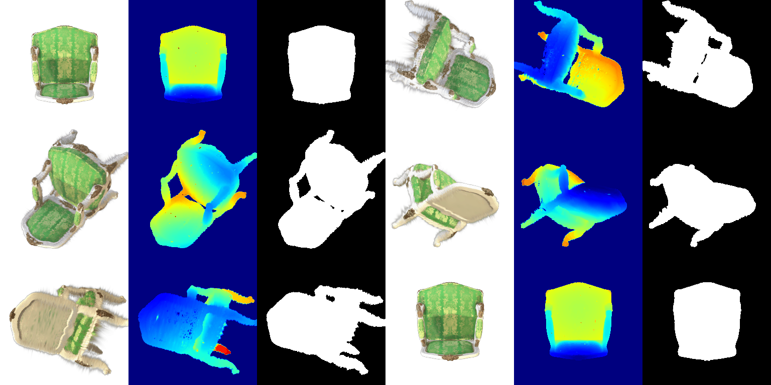
Pre-trained chair: color, depth and mask (render.py, DC color only)
Isotropic Gaussians initialized from the truck point cloud, L1 loss, Adam with a separate learning rate per parameter, 1000 iterations. The means get by far the smallest step: they are in scene units and a small move changes the image substantially (with the starter's 0.05 everywhere the render actually turns to confetti within a few iterations). Opacities and colors are bounded by their activations and can move fast.
| Parameter | Learning rate |
|---|---|
| opacities | 0.05 |
| scales | 0.005 |
| colors | 0.02 |
| means | 0.0005 |
| Truck, held-out views | PSNR | SSIM |
|---|---|---|
| 1000 iterations | 29.39 | 0.938 |
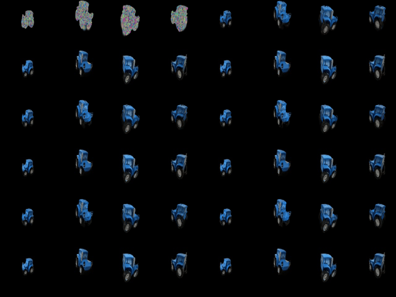
Training progress (top: render, bottom: ground truth)

Final renders of the training views
How: for each Gaussian, the direction from the camera center to its mean is normalized and all 16 spherical-harmonic coefficients per color channel (degree 3) are evaluated in that direction. With only the constant term this reproduces the question 5 colors exactly.
Q5: DC color only
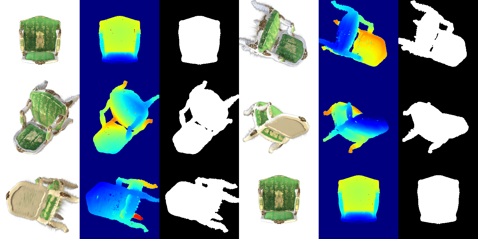
Q7.1: full spherical harmonics
Same views side by side, DC only on the left, full SH on the right:

View 4 (three-quarter from above): with SH the green fabric is more saturated and darker in the folds, and the gold embroidery on the backrest picks up highlights instead of a flat tint. The DC render looks evenly lit and a touch gray.

View 12 (looking down at the seat): the clearest difference. The seat cushion gets a soft sheen towards the camera and the trim on the armrests shifts color with the angle; DC keeps the average color and looks washed out.

View 20 (from below): almost no difference. The underside is matte and was probably seen from few directions in the original training, so the higher-order coefficients carry little there.
The geometry is identical in both renders, only the per-Gaussian color changes, so every difference is shading. On this mostly matte chair the effect is admittedly subtle; on a glossy object the DC-only render would be visibly wrong.
Materials scene, 10,000 Gaussians at random inside a small sphere (the given
init_type="random"), 128x128 renders.
Baseline: the question 6 recipe unchanged (isotropic, L1, the same learning rates, 1000 iterations).
Improved, every change relative to question 6:
| Materials, 100 held-out views | Iterations | PSNR | SSIM |
|---|---|---|---|
| baseline (Q6 setup, random init) | 1000 | 18.14 | 0.679 |
| improved | 3000 | 19.61 | 0.784 |
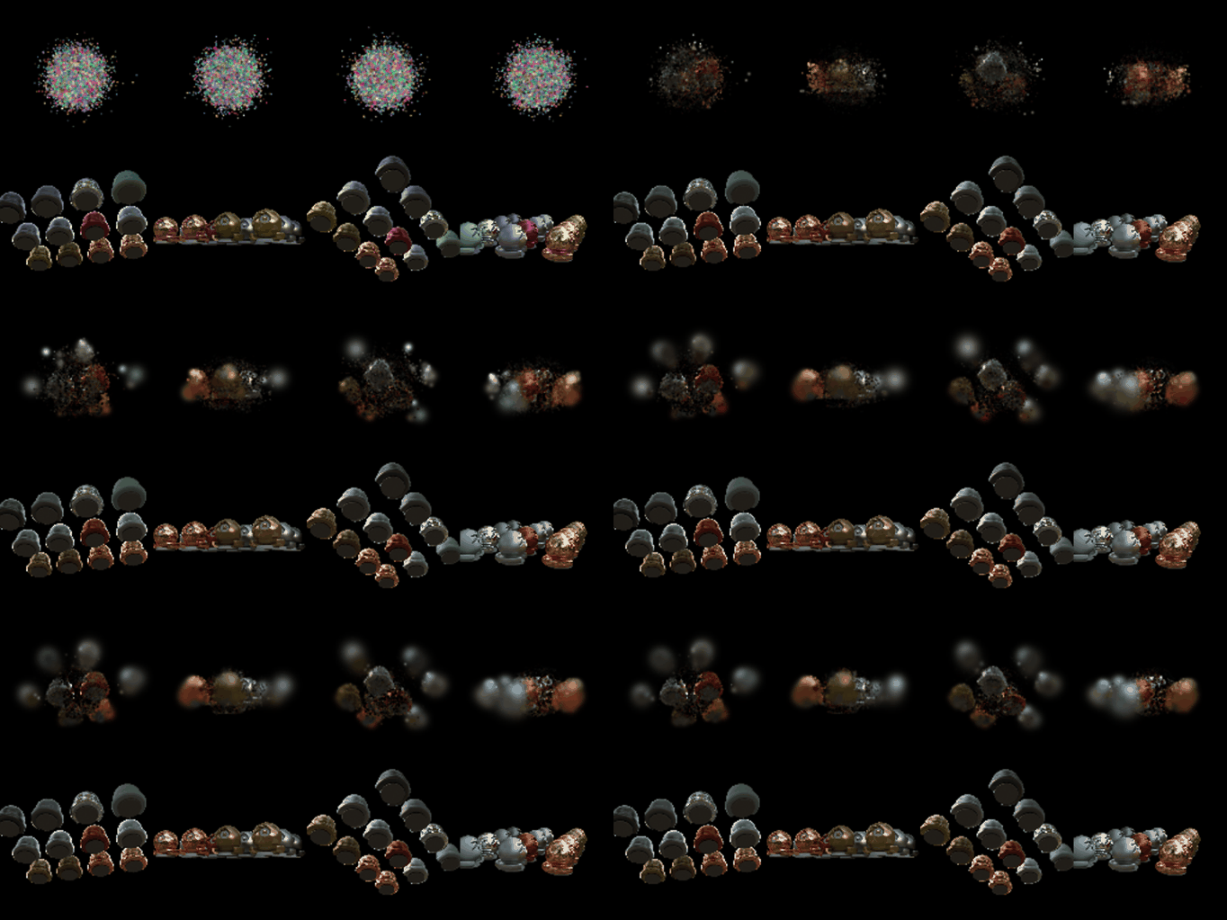
Baseline: training progress
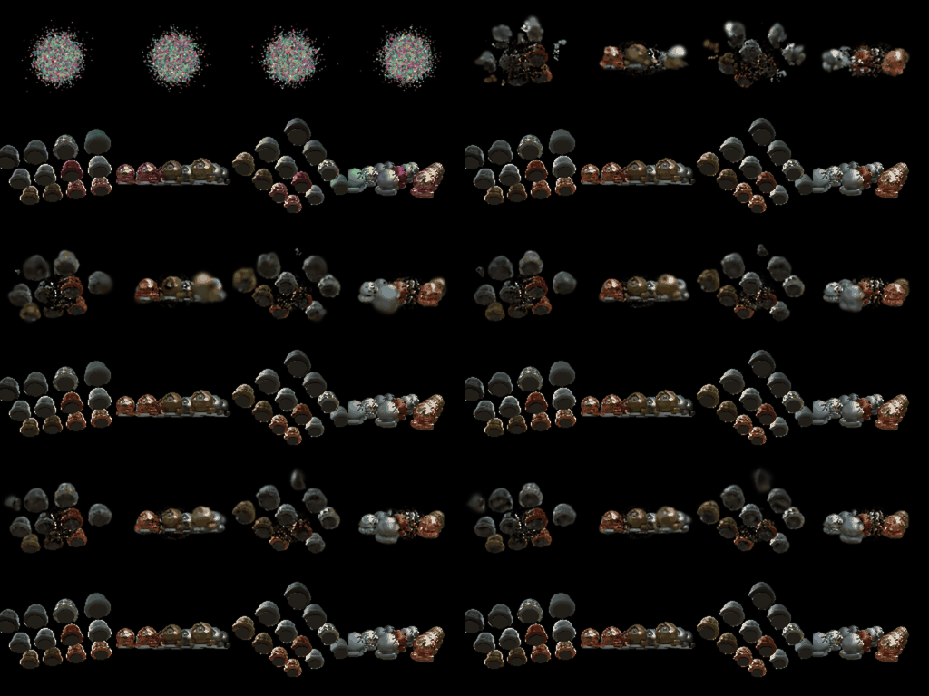
Improved: training progress

Baseline: final renders
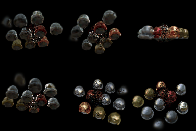
Improved: final renders
The baseline never gets past one blurry cloud per cluster of spheres: with isotropic blobs started at random and a plain L1 loss, smearing the average color over the right region is actually the cheapest solution, and with the small means learnign rate the Gaussians cannot leave the initial ball in 1000 iterations. The improved run resolves the individual spheres, their colors and the ground plane. SSIM moves substantially more than PSNR (+0.1 vs +1.5 dB) because the extra loss term optimizes exactly that. It is still soft, and a few dark Gaussians float between the spheres in some views, which the real method would remove with its opacity reset and split step. Consequently, the biggest remaining lever is the initialization itself: most of the 3000 iterations seemingly go into moving Gaussians out of the small start sphere into the scene at all, so a wider init (or points from the 4.1 NeRF) would help more than any of the changes above.