
Binary cross entropy with logits on the 32x32x32 grid.
Fitted voxel grid (left) vs target (right)
Chamfer distance implemented with two knn_points(K=1) calls (source to target and target to source), squared distances summed over points.
Fitted point cloud (left) vs target (right)

Laplacian smoothing: the uniform laplacian of the vertices as a smoothing term. This was combined with chamfer from previous section, w_smooth = 0.1.
Fitted mesh (left) vs target mesh (right, green)

The voxel decoder starts from the 512-d image feature, expands it with a linear layer into a small 256-channel 2x2x2 volume, and then doubles the resolution four times with transposed 3D convolutions (each followed by batch norm and ReLU) until it reaches 32x32x32, where a final 3x3x3 convolution produces one occupancy logit per cell. It is trained with the binary cross-entropy from 1.1, but with the occupied cells weighted three times more than the empty ones -- about 96% of the grid is empty, so with plain BCE the network learns that "predict nothing" is a safe answer and drops the legs, which gives 57.8 instead of 69.9. For the renders and the F1 score the logits go through a sigmoid and marching cubes at 0.5, in the same frame as the ground-truth mesh.
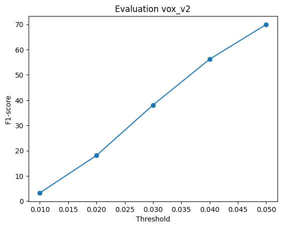
F1@0.05 = 69.9
Three test examples. Each panel is: input RGB | predicted voxel grid | ground truth mesh.
Example 1

Example 2
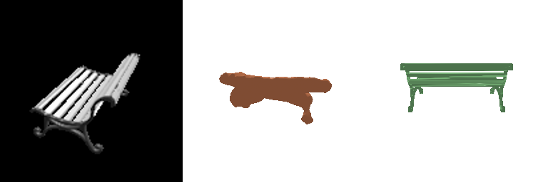
Example 3
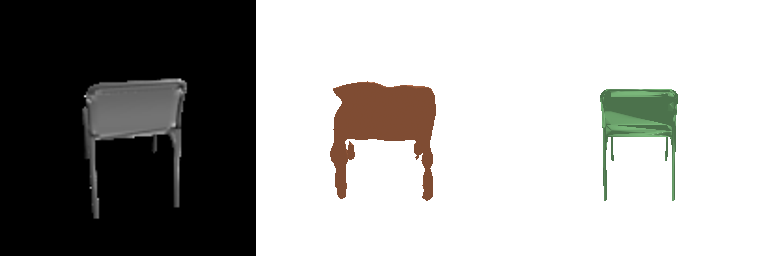
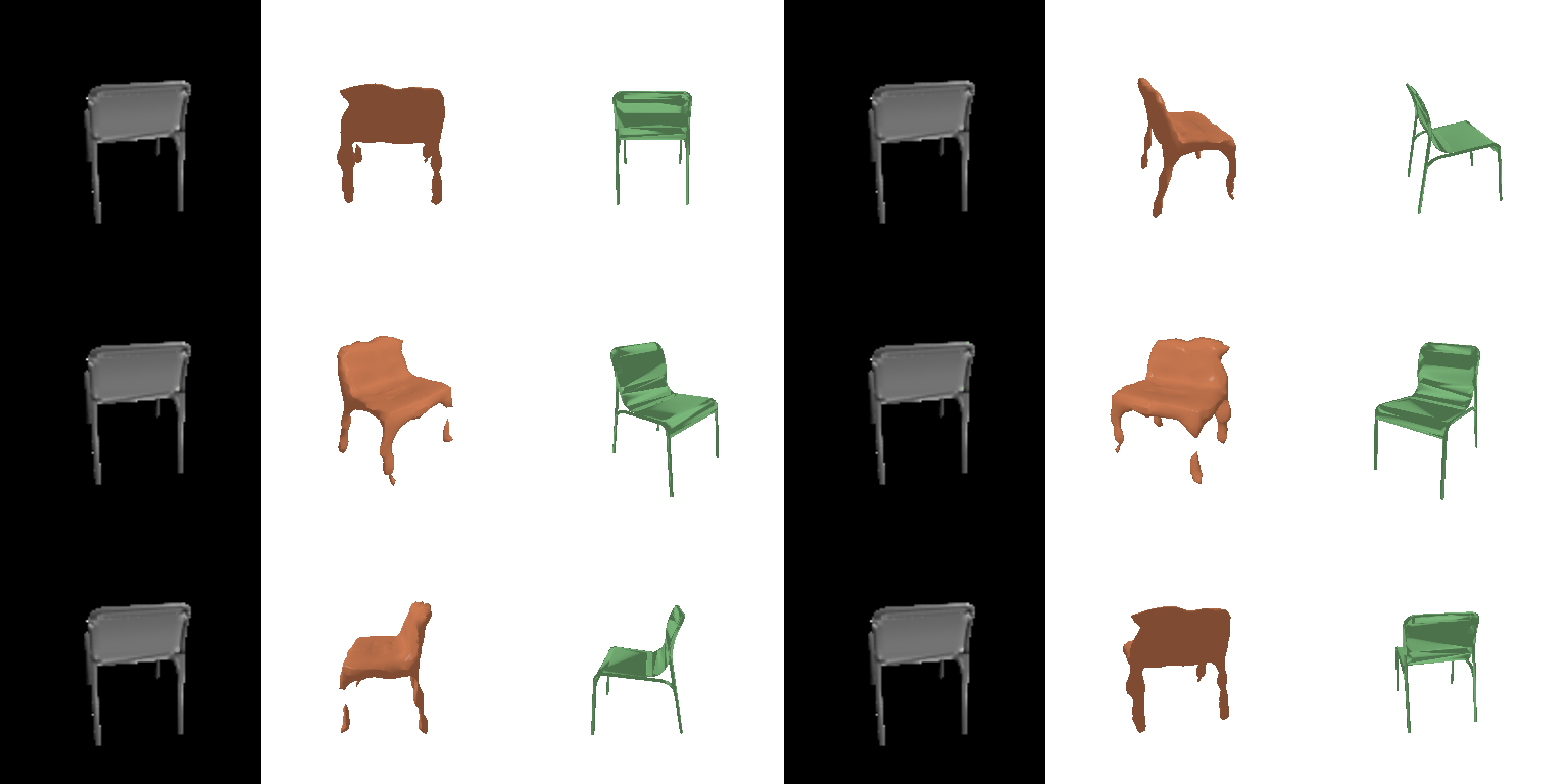
Turntable of example 1 (input | prediction | ground truth)

Turntable of example 3
F1 vs threshold on the full test set
The point decoder is a plain MLP, (512, 1024, 2048, 3x2000), with leaky ReLU in between and a tanh on the output so the coordinates stay in the range the ShapeNet meshes occupy. It is trained with the Chamfer loss from 1.2 against 2000 points sampled from the ground-truth mesh.
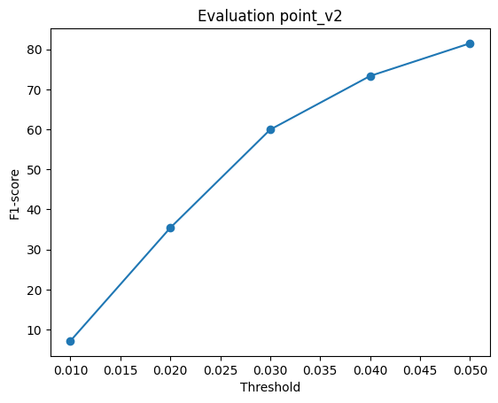
F1@0.05 = 81.5
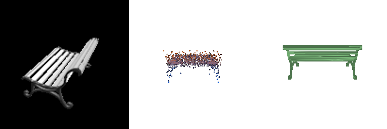
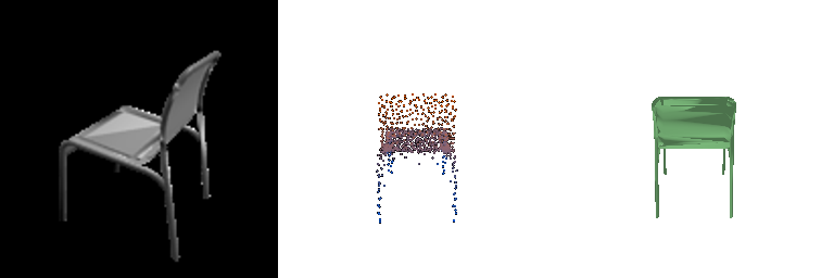
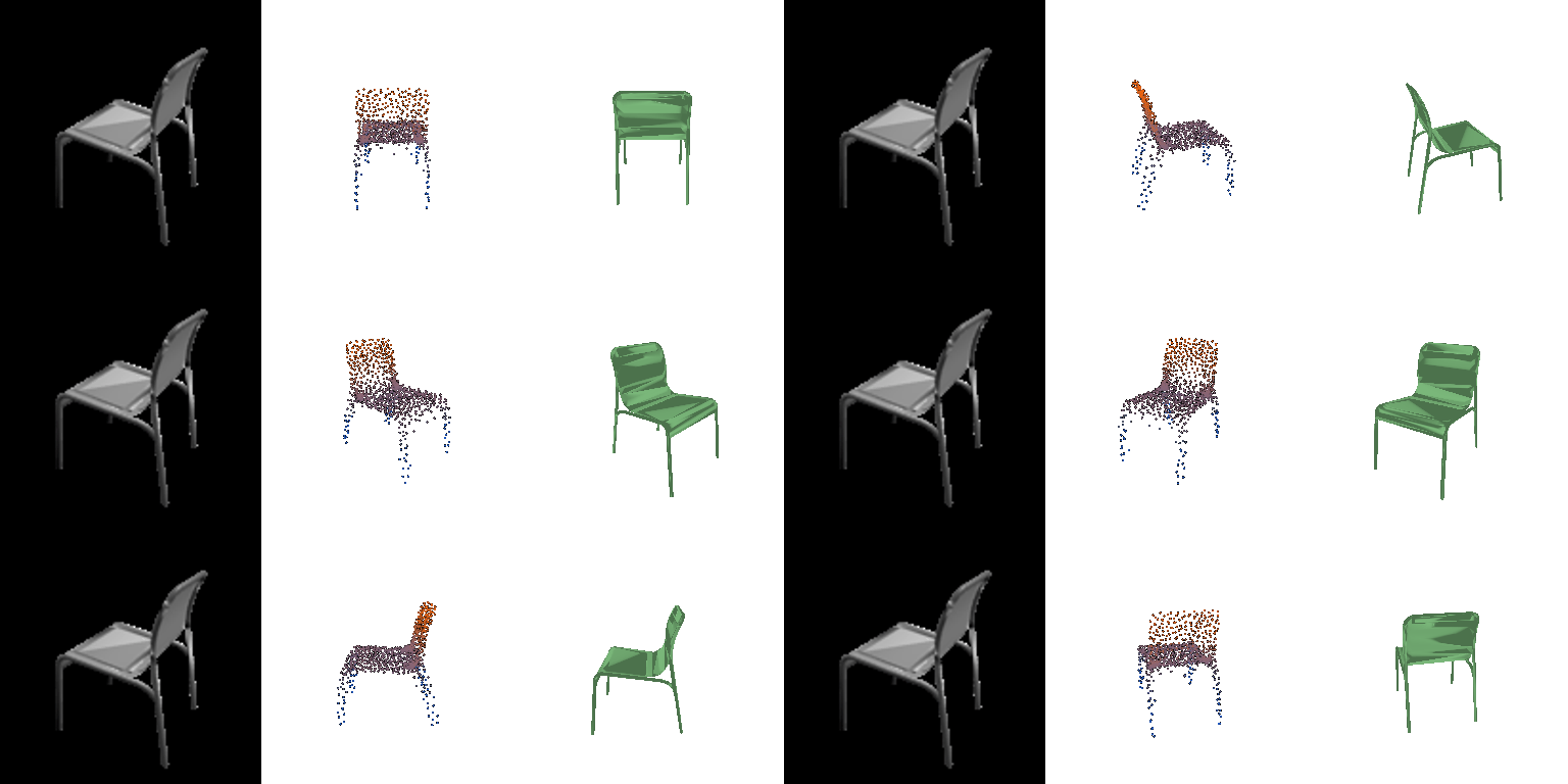
Three test examples. Each panel is: input RGB | predicted point cloud | ground truth mesh.
Example 1

Example 2
Example 3
Turntable of example 1 (input | prediction | ground truth)

Turntable of example 3
F1 vs threshold on the full test set
The mesh decoder has the same MLP shape as the point decoder but its 3x2562 outputs are read as an offset for every vertex of an ico_sphere(4) template, with a tanh keeping the offsets bounded, so the prediction is always that sphere pushed and pulled into a chair. Both the predicted and the ground-truth surfaces are sampled at 1000 points for the Chamfer loss from Q1.2, and the Laplacian smoothness loss from Q1.3 is added with weight 1 to stop neighbouring vertices from flying apart.
F1@0.05 = 75.4
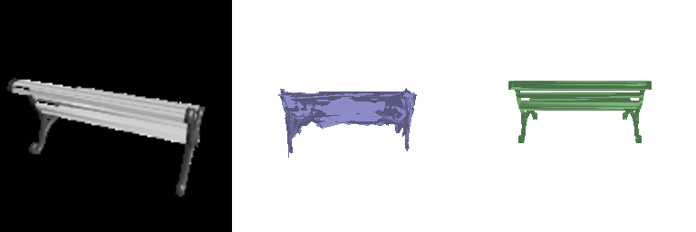
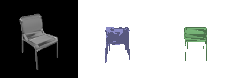
Three test examples. Each panel is: input RGB | predicted mesh | ground truth mesh.
Example 1

Example 2
Example 3
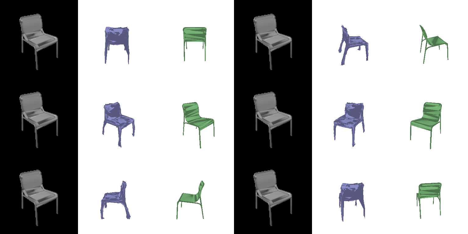
Turntable of example 1 (input | prediction | ground truth)

Turntable of example 3
F1 vs threshold on the full test set
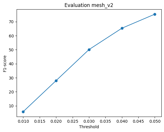
Point clouds came out on top at 81.5, meshes in the middle at 75.4, and voxels last at 69.9. The ordering makes sense -- the more structure a representation has, the more it can capture the underlying shape. A point cloud has no structure to respect at all: every point is placed independently, so a few of them can go off and form a leg or an armrest without dragging anything else along. On top of that it is trained directly on Chamfer loss. Both F1 score and chamfer distance measure bidirectional geometric agreement, so the model is optimising almost exactly what we score it on. The mesh is held back by its starting shape. Everything it produces is a warped sphere, which means it can never open a hole between the legs or through the back of the chair. Those regions end up bridged by stretched triangles, and any point sampled from that bridge is obviously a false positive. The Laplacian term makes it a little worse for thin parts, since it actively discourages the sharp bends a leg or a slat would need. Voxels sit at the bottom mostly because 32 cells per side is just not enough for chair legs, which end up one cell wide and often vanish once you threshold at 0.5. The loss doesn't help either -- cross-entropy evaluates every voxel separately so there is no real geometric structure to it.
n_points for the point decoder (5k iterations each):
| n_points | 500 | 1000 | 2000 | 5000 |
|---|---|---|---|---|
| F1@0.05 | 73.9 | 79.9 | 85.5 | 88.2 |
F1@0.05 vs n_points

More points cover a larger surface area which pushes the recall up, thereby increasing the F1 score as well. The evaluation also samples n_points from the ground truth so denser ground truth helps precision too.
a. View consistency: the same object through all 10 of its test views. F1 varies from 31 to 89 for the armchair (back views occlude the legs), so there is extreme view dependence. The model seemingly focuses on the silhouette and guesses the rest of the object.
Top row: the 10 input views, bottom row: the mesh predicted from each

F1@0.05 per view

b. Latent interpolation between two test chairs, decoded with the point model. The intermediate shapes are all plausible chairs, so the decoder has actually learnt a smooth chair space!
Interpolation 1 (left image, six decoded steps, right image)

Interpolation 2

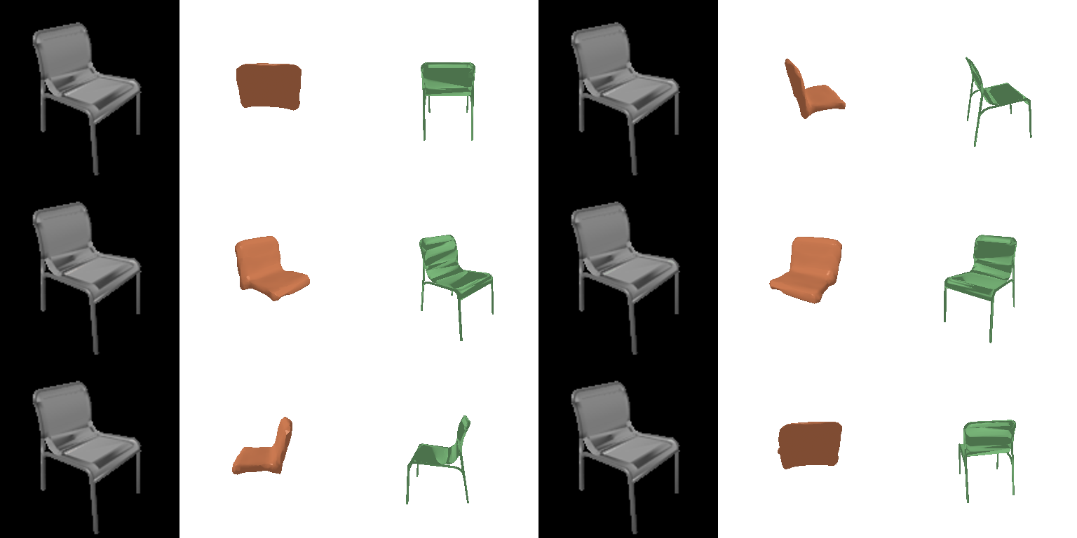
The implicit decoder takes the image feature and a single 3D coordinate, projects each to 256 dimensions, adds them, and runs a three-hidden-layer MLP to get one occupancy logit for that location. Evaluating it on a 32x32x32 grid over (-1, 1)^3 gives back the same kind of grid as the voxel model, so the loss, ground truth and evaluation are unchanged, only now a 0.3M-parameter network is shared across all locations instead of a 3.8M-parameter convolutional stack generating everything at once. It scores 62.0 against 57.8 for the convolutional decoder with the same plain BCE, with smoother outputs because occupancy is continuous in position, at the cost of the thin legs, for example, being smoothed away.
Example 1 (input | predicted occupancy | ground truth)

Example 2
F1 vs threshold

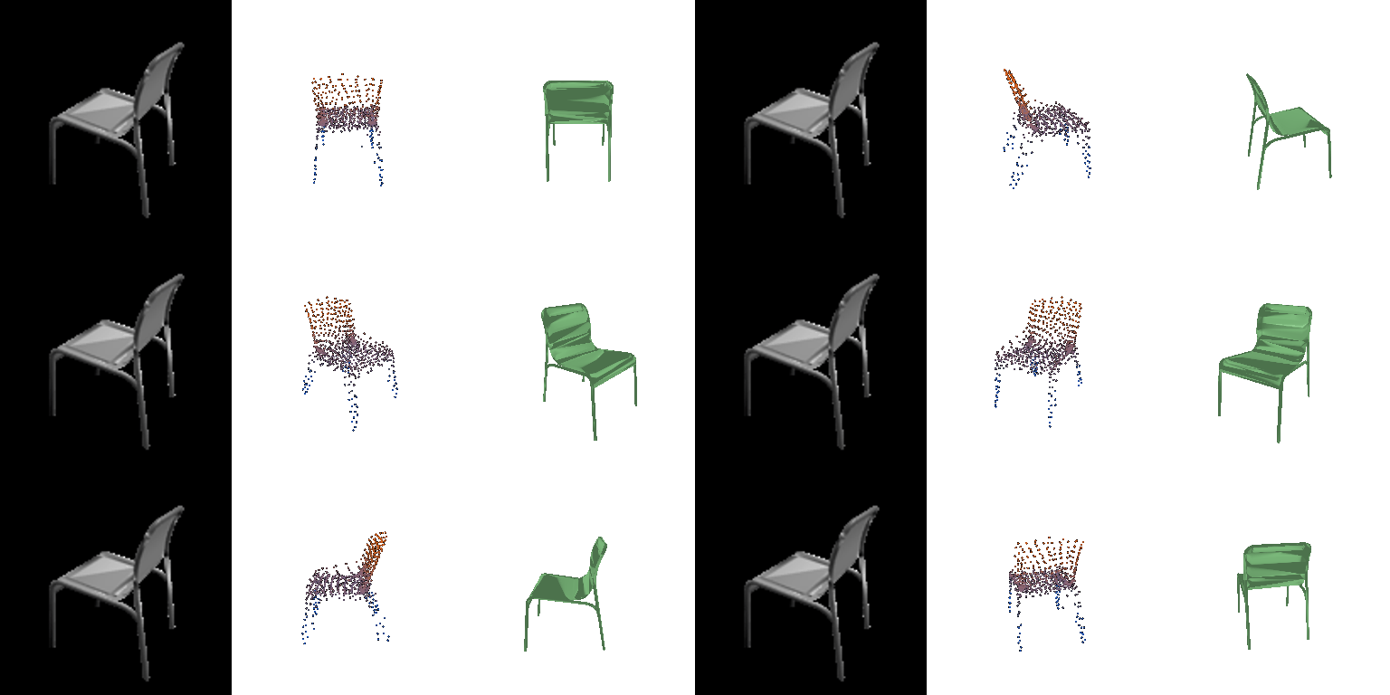
The parametric decoder maps a 2D coordinate in the unit square, concatenated with the projected image feature, through a (512, 256, 128, 3) MLP with tanh output, so sampling many (u, v) pairs traces out a surface. I used four such patches, with random uv during training and a 15x15 grid per patch at test time, trained with the same Chamfer loss as the point model. It scores 76.6 against 79.9 for the plain point decoder, because every point must lie on one of four continuous sheets and its hard to wrap a chair with legs and back using 4 patches. An important advantage of this method is that the number of output points isn't fixed by the architecture, and the uv grid gives a triangulation for free.
Example 1 (input | predicted point cloud | ground truth)

Example 2
F1 vs threshold

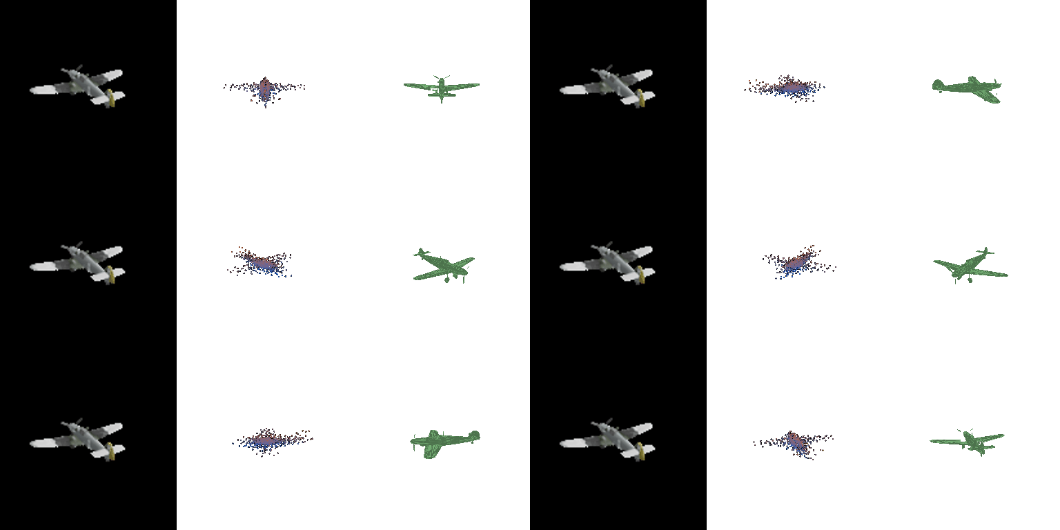
Point and mesh models trained on chair + car + plane, 10k iterations, and the chair-only models evaluated on the same 3 class test split (1451 models).
| model | chair F1 | car F1 | plane F1 |
|---|---|---|---|
| point, trained on chairs | 79.8 | 66.9 | 74.2 |
| point, trained on 3 classes | 81.2 | 92.8 | 96.4 |
| mesh, trained on chairs | 76.0 | 69.3 | 65.3 |
| mesh, trained on 3 classes | 75.8 | 91.5 | 95.0 |
Each panel: input | prediction | ground truth.
Plane, point model trained on chairs only

Plane, point model trained on 3 classes
Car, mesh model trained on chairs only

Car, mesh model trained on 3 classes

Chair, point model trained on chairs only

Chair, point model trained on 3 classes

Chair F1 does not drop when training on three classes (79.8 to 81.2 for points) even though the model sees a third as many chair batches. Cars and planes are much easier since they are compact, near convex, and more consistent within class. The chair-only model outputs chair shaped blobs for planes and cars; its 65 to 74 there is only because everything is normalised into the same box.As expected, the 3 class model's outputs better reflect the respective class-shapes.