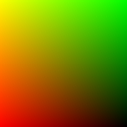
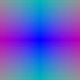
The left image is the xy grid from vis_grid and the right image is the ray directions from vis_rays for the first camera, and both match the TA images. I mapped the pixel coordinates to [-1, 1] so the corner pixels land exactly on -1 and 1, since sample_images_at_xy uses align_corners=True. Then I put every pixel on the image plane at depth 1, unprojected it to world space with camera.unproject_points, and took the direction from the camera center to that point. I normalized the directions so that the distances along a ray are real world distances.
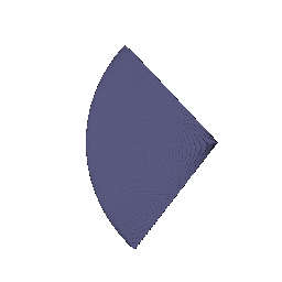
These are the sample points from the first camera rendered with render_points. The sampler puts 64 evenly spaced points on every ray between the near depth (0) and the far depth (5). The fan shape is the camera frustum seen from the side, and the far edge is rounded because every ray stops at the same distance from the camera instead of at the same depth plane.
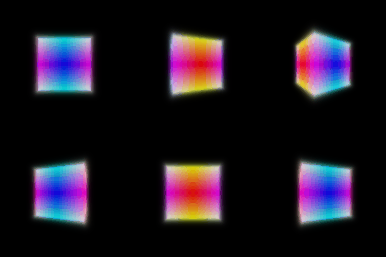

Depth from camera 2
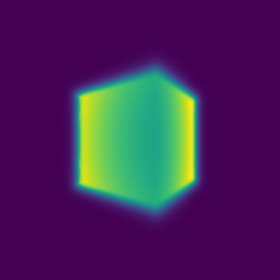
The top left is the rendered box and the top right is its depth from the same cameras, and the bottom image is the depth from camera 2, normalized by its max. For every ray segment the opacity is 1 - exp(-sigma * dt), the transmittance T is the product of (1 - opacity) over all the segments before it (so T = 1 for the first one), and the weight is T times the opacity. The color is the sum of weight * color and the depth is the sum of weight * distance, so the depth is basically the expected distance where the ray gets absorbed. Rays that miss the box have weights close to 0, which is why the background depth is 0. The edges of the box are soft because the SDF is turned into density with beta = 0.05, so the density ramps up over a small distance outside the surface instead of jumping.
For each training step I take 4096 random pixels out of the 65,536 pixels in one image. I shuffle all the pixels with torch.randperm and keep the first 4096 so the same pixel is never picked twice in a batch.
Box center: (0.25, 0.25, 0.00)
Box side lengths: (2.01, 1.50, 1.50)
The loss is the mean squared error between the rendered colors and the ground truth colors at the sampled pixels. The box starts as a 1.5 x 1.5 x 1.5 cube at the origin and training takes about 25 seconds for 1000 epochs, ending at an MSE of about 1e-6. I got the same numbers to 3 decimal places in three different runs.
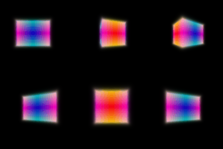
My spiral rendering (left) vs the TA's (right)
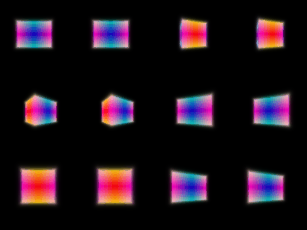
My gif matches the TA's. Over the 20 frames the average difference is 0.7 / 255 per pixel, and only about 1% of the pixels are off by more than 30 / 255. Those pixels are all inside the rainbow part of the box and none of them are in the background, so I think it is just the two gifs picking different 256 color palettes for the same gradient and not a difference in the box itself.
Ground truth, before training, after training
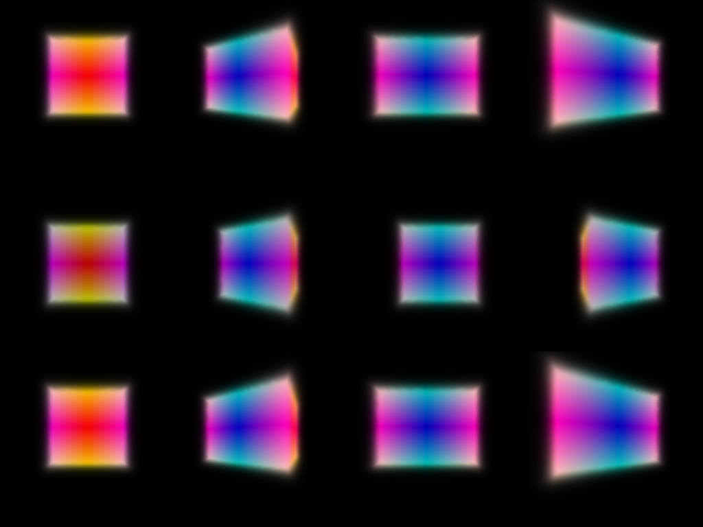
The columns are the 4 training cameras. Before training the box is too narrow along x and sits at the origin. After training it grew along x and moved up and to the side, which is easiest to see in the two diagonal views (columns 2 and 4), and the renders match the ground truth to within 0.3 / 255 per pixel.
Validation PSNR = 24.4 dB
Mine (left) vs the TA's (right)
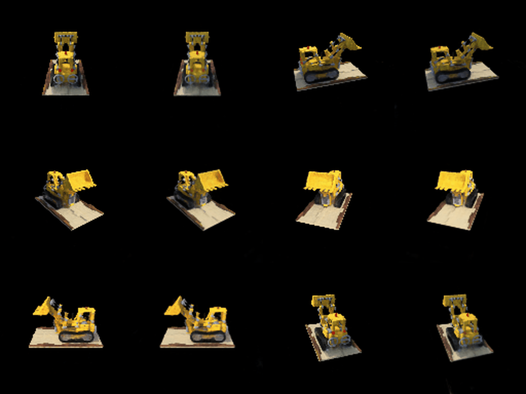
My NeRF looks the same as the TA's. The bucket, the treads and the base plate are all there with about the same amount of blur at 128 x 128.
The MLP takes the positional encoding of each point (6 frequencies, so 39 numbers) and passes it through 6 linear layers of width 128 with ReLUs, and the encoding gets concatenated back in before the 4th layer like the skip connection in the NeRF paper. From the 128 dimensional feature, one linear layer and a ReLU give the density, and a small head (128 to 64 to 3) with a sigmoid gives the color. For this part the color only depends on position and not on the viewing direction. I trained with the default nerf_lego.yaml settings (250 epochs, 128 x 128 images, 128 samples per ray between depth 2 and 6), which took about 5 minutes on my RTX 5090. The PSNR is the average over the 100 validation views (between 22.1 and 26.6 for single views) using the epoch 200 checkpoint, which is the last one the code saves.
I did all three extras. All of the PSNRs here are on held-out validation views that the model never trained on, unless I say train.
Materials at 400 x 400: validation PSNR 24.4 dB with view dependence and 23.5 dB without
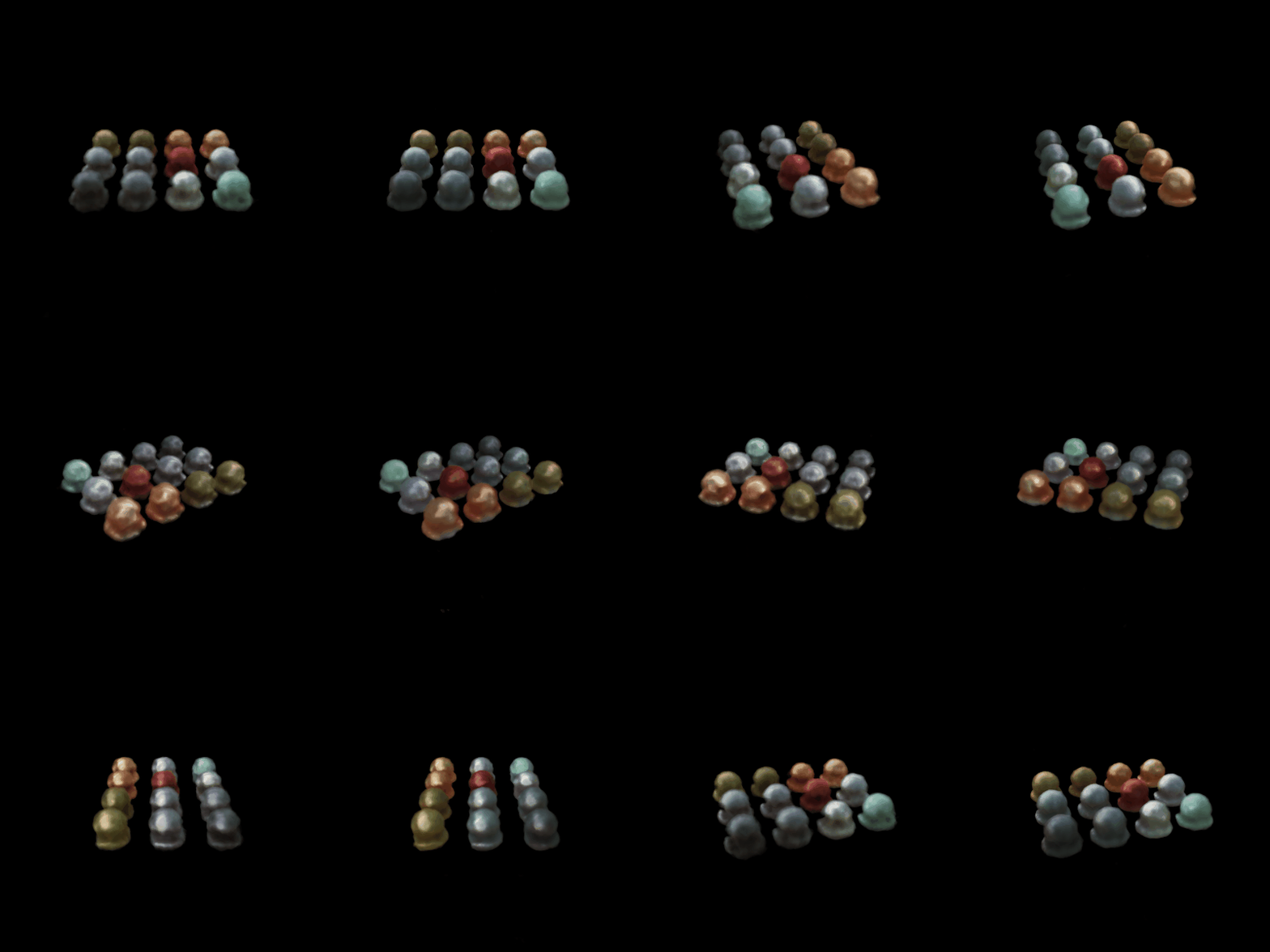
These are nerf_materials_highres.yaml without view dependence (left) and with view dependence (right).
Ground truth, without, with


Neither model gets the sharp mirror reflections from the ground truth and both are blurry, but they fail differently. Without view dependence a point on a shiny sphere has to have the same color from every direction, but the training images show it bright from some directions and dark from others. The network can't fit both, so the spheres come out mottled and fuzzy at the edges. With view dependence the color can change with the direction, so the spheres come out smooth and closer to the right colors.
To add view dependence I only feed the viewing direction into the color part of the network. The trunk and the density are the same as in part 3. For the color, the feature goes through one more linear layer, I concatenate the positional encoding of the ray direction (2 frequencies) to it, and then a 64 wide layer and a sigmoid give the RGB. This is how the NeRF paper does it: density only depends on position, so the geometry is the same from every direction, and only the color is allowed to change with view.
View dependence vs generalization
To look at the trade-off, I trained four versions on materials at 128 x 128, once with all 100 training views and once with only 20 of them (trained 5x longer so every run takes the same number of steps). The gap is train PSNR minus validation PSNR, which shows how much better a model does on the views it trained on than on new ones. I ran the 20 view versions with direction in the color head twice and the table has the average.
| Model | 100 views: val PSNR | 100 views: gap | 20 views: val PSNR | 20 views: gap |
|---|---|---|---|---|
| No view dependence | 23.5 | 0.13 | 22.9 | 1.27 |
| Direction in the color head, 2 frequencies | 24.4 | 0.19 | 23.7 | 1.15 |
| Direction in the color head, 6 frequencies | 24.3 | 0.19 | 23.6 | 1.31 |
| Direction in the color head and the trunk (density depends on view too) | 24.7 | 0.31 | 23.0 | 2.36 |
Models trained on 20 views, on held-out views
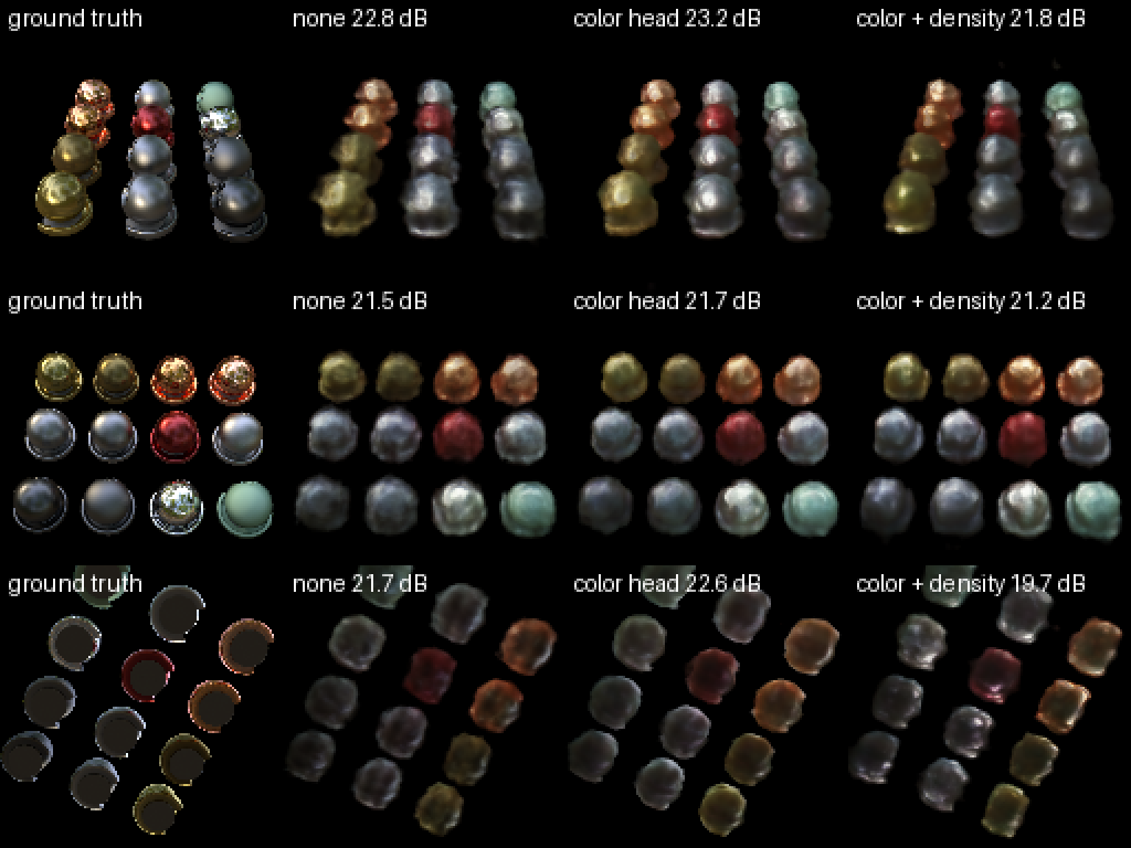
Some view dependence helps a lot on this scene because it is full of glossy and metal spheres whose color really does change with view. Putting the direction in the color head gains about 0.9 dB with 100 views and 0.8 dB with 20 views, and the gap doesn't get bigger.
But the more freedom the network has to explain a pixel with its viewing direction instead of the actual 3D scene, the more it fits the training views and the worse it does on new ones. With 6 frequencies the color can change faster with direction, and the gap grows a little (1.15 to 1.31 with 20 views) without doing any better on new views. When I also put the direction into the trunk, the density can change with view too, so each training image can basically get its own version of the geometry. With 20 views that version has the best train PSNR of everything (25.3) but the worst validation PSNR of the view dependent models (23.0), and the gap is twice as big. In the panel above it is the worst one on all three views, especially the third one (19.7 dB), where its spheres come out darker and more mottled.
How much this matters depends on the number of views. With 100 views every direction around a point gets seen enough that even the trunk version is held in place, and it is actually the best on validation (24.7). With 20 views most directions are never seen, and the extra freedom just goes into memorizing the training images. So the safe choice is what the NeRF paper does, which is density from position only and the direction only in a small color head with a low frequency encoding.
One thing that went wrong along the way: in my first round two of the three 100 view runs came out almost completely black (val PSNR around 15). When I looked into it, the raw density at initialization is almost the same everywhere and its sign comes from the random bias of the last layer. If it starts negative, the ReLU makes the density 0 everywhere, the gradient is 0 everywhere, and the network never recovers. This happened for 2 out of the 5 random seeds I checked, so I initialized that bias to 0.1 so every point starts with a small positive density. All of part 4 uses this fix (the part 3 lego run was before the fix and just got lucky). One 20 view run without view dependence still came out broken after the fix (val 14.6, mostly black with floaters), so I reran it and the table uses the rerun.

| Sampling (lego, 128 x 128) | Network evaluations per ray | Val PSNR | Render time per image | Training time for 11 epochs |
|---|---|---|---|---|
| Uniform 64 | 64 | 23.4 | 12 ms | 7 s |
| Uniform 128 | 128 | 24.6 | 23 ms | 9 s |
| Uniform 256 | 256 | 25.0 | 49 ms | 16 s |
| Coarse/fine 32 + 32 | 96 | 24.2 | 18 ms | 12 s |
| Coarse/fine 64 + 64 | 192 | 24.9 | 37 ms | 12 s |
| Coarse/fine 64 + 128 | 256 | 24.9 | 49 ms | 14 s |
Coarse/fine 64 + 128 means the coarse network looks at 64 points and the fine network looks at those 64 plus 128 new ones, so it costs 64 + 192 = 256 network evaluations per ray. Everything was trained for 250 epochs with the nerf_lego.yaml settings, and all of them (uniform too) jitter their samples randomly inside their bins during training. Without the jitter uniform 128 gets 24.5 dB, so the jitter by itself doesn't change anything here. I timed everything with nothing else running on the GPU.
I used two separate NeRF networks with the same architecture as part 3. For each ray the coarse network is rendered at the usual stratified samples, and its weights get normalized into a probability distribution along the ray. I draw the new fine depths from that distribution with inverse transform sampling (randomly during training and evenly spaced when rendering), and the fine network is rendered at all the coarse and fine depths sorted together. Both networks get the MSE loss against the ground truth, and only the fine network is used for the final image.
Where the samples go on one ray
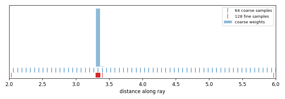
This is one ray that hits the bulldozer. Almost all of the coarse weight is in one bin at the surface, about 3.3 units from the camera, so almost all of the 128 fine samples land in that one bin, which is only 0.06 units wide. The uniform samples are spread across the whole range from 2 to 6, and most of them are in empty space where they don't add anything to the color.
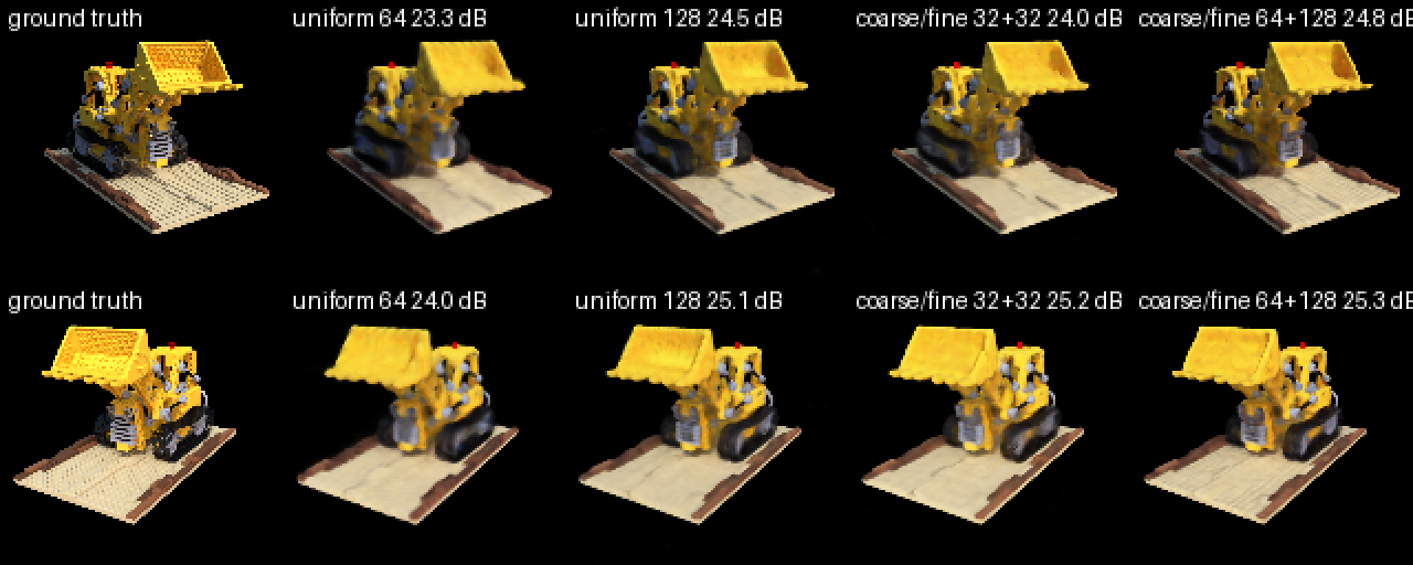
Coarse/fine is a lot better when you can't afford many samples. With 96 evaluations it gets 24.2 dB, which is close to uniform 128 (24.6) and way above uniform 64 (23.4), and in the two views above uniform 64 is the blurriest one. But once there are more than about 150 evaluations the two curves meet, and at 256 uniform is even slightly ahead (25.0 vs 24.9). I think this is because lego is a small object with tight near and far bounds (2 to 6), so 128 to 256 uniform samples already put a few samples on every surface, and the limit becomes the 128 x 128 images and the network size instead of where the samples are. Coarse/fine should matter more for scenes with a bigger depth range or thin things that uniform samples can step over.
Render time goes almost exactly with the number of evaluations for both, since the sorting and sampling are cheap, so coarse/fine 64 + 128 and uniform 256 both take 49 ms. Training is a different story. With only 1024 rays per step the GPU isn't fully used, so running two networks plus the sampling step adds overhead, and coarse/fine 32 + 32 actually trains slower than uniform 128 (12 s vs 9 s for 11 epochs) even though it evaluates fewer points. It also has twice the parameters, and the coarse network is only there to place samples. So coarse/fine gets you more quality for the same render time (almost uniform 128's quality, 24.2 vs 24.6 dB, for 78% of its render time), but it costs memory, training time and complexity, and on a small scene like this just taking more uniform samples works as well once the budget is big enough.
Best result: validation PSNR 24.1 dB (sphere initialization, Softplus, alpha = 50, beta = 0.02, everything else from volsdf_surface.yaml. The default config gets 22.0 dB)
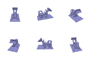
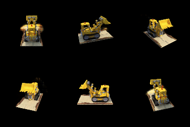
My geometry, the TA's geometry, my color, the TA's color
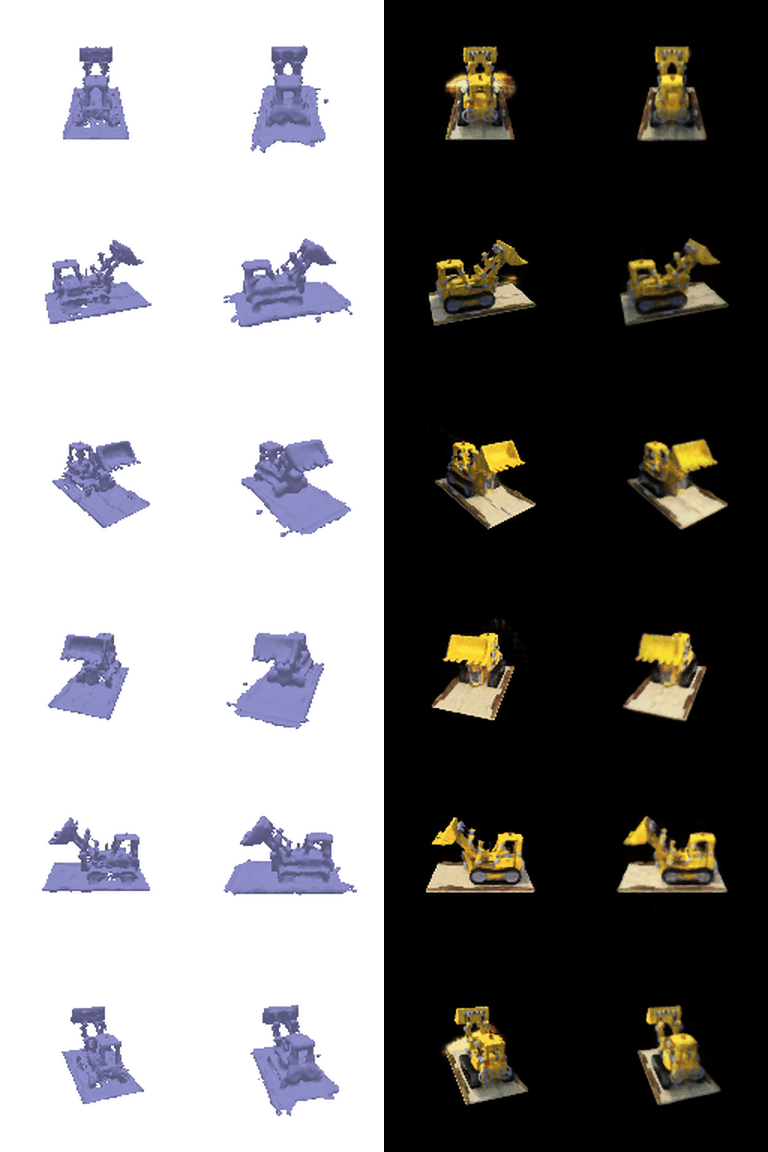
The geometry is the zero level set of the SDF from marching cubes. Mine has the same shape as the TA's and is a little sharper in the thin parts (the arm, the bucket and the cab pillars), with a thinner and flatter base plate.
For the distance I encode the position with 6 frequencies and use an MLP with 6 layers of width 128 that outputs 129 numbers. The first one is the signed distance, which has no activation at the end because a distance can be negative (unlike density, which has a ReLU), and the other 128 are a feature for the color like in IDR and VolSDF. The color is a 2 layer MLP that takes the feature and the encoded position and outputs RGB with a sigmoid, and get_distance_color runs the distance network once and uses it for both. The eikonal loss is the mean of (|gradient of d| - 1)^2 at 1024 random points in the [-4, 4] box, since a real SDF has a gradient of length 1 everywhere. For the density I used the VolSDF formula, density = alpha * Psi_beta(-d), where Psi_beta is the CDF of a Laplace distribution with scale beta. That works out to alpha * (1 - 0.5 exp(d / beta)) inside the object and alpha * 0.5 exp(-d / beta) outside.
What alpha and beta do
Alpha is the density deep inside the object. The density is alpha / 2 right at the surface, goes up to alpha inside and goes down to 0 outside, so alpha controls how solid the object is. My samples are about 0.03 apart, so one sample inside the object blocks 1 - exp(-alpha * 0.03) of the light, which is 27% for alpha = 10 and 79% for alpha = 50. Beta controls how wide the change from empty to solid is. The density changes by a factor of e every beta of distance, so it goes from full to almost nothing over a band a few beta thick around the surface. Small beta gives a sharp surface and big beta gives a soft, foggy one, and as beta goes to 0 the density becomes alpha inside the object and 0 outside.
1. How does high beta bias your learned SDF? What about low beta?
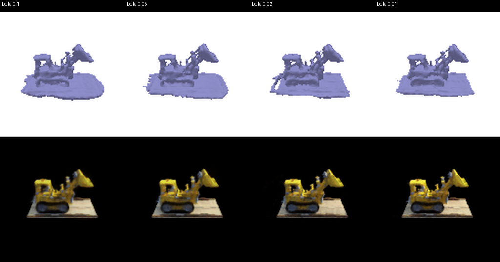
With high beta the density leaks pretty far out from the surface, so a ray picks up a lot of opacity before it even reaches the zero level set. To match the images the network has to make the SDF smooth and round, so the surface you actually see sits outside the zero level set, and sharp corners and thin parts get spread out or disappear. In my beta = 0.1 model the base plate is puffed up with rounded edges, and its mesh has the most area of my Softplus models (17.4 vs 14.7 for the final one). With low beta the density is almost a step at d = 0, so the opacity comes almost entirely from the zero crossing and the zero level set gets pushed to exactly where the images say the surface is. The bias then goes the other way: the SDF is only pinned down in a really thin band around the surface, and away from it only the eikonal loss shapes it, so it can have extra zero crossings (floaters) that the images don't punish.
2. Would an SDF be easier to train with volume rendering and low beta or high beta? Why?
High beta. The gradient of the density with respect to d is (alpha / 2 beta) exp(-|d| / beta), which is basically 0 more than a few beta away from the surface. With high beta, points far from the current surface still get a gradient, so a surface in the wrong place can get pulled a long way and training is smooth. With low beta only the samples that land in a really thin band get any gradient (beta = 0.01 is only a third of my sample spacing), so the signal is sparse and noisy, and parts of the scene that start in the wrong place might never get fixed. My runs without the sphere initialization show this: beta = 0.01 ended up with 7474 separate mesh pieces and 40% of the mesh area in floaters, while beta = 0.2 had 260 pieces.
3. Would you be more likely to learn an accurate surface with high beta or low beta? Why?
Low beta, as long as training is kept stable some other way. As beta goes to 0 the density becomes exactly the inside of the object, so the surface you render and the zero level set become the same thing, while high beta can never make a sharp edge or a thin part no matter how long it trains. My best geometry is at low beta (0.02) and it is the sharpest in the thin parts. VolSDF itself starts with a large beta and makes it smaller during training (they actually learn beta), and here the sphere initialization is what lets me use a small beta from the start.
Hyper-parameter experiments
Everything was trained on lego for 250 epochs at 128 x 128. Besides PSNR I also looked at the extracted mesh: how many separate pieces it has (bigger than 0.001 in area) and how much of the total area is in the biggest piece, since anything outside the main piece is a floater.
| Settings | Val PSNR | Mesh pieces | Area in main piece | Total mesh area |
|---|---|---|---|---|
| Default config (alpha 10, beta 0.05, eikonal 0.02, ReLU) | 22.0 | 522 | 91.9% | 403 |
| eikonal weight 0.1 | 21.3 | 1070 | 87.6% | 179 |
| beta 0.01 | 22.5 | 7474 | 60.1% | 526 |
| beta 0.2 | 20.2 | 260 | 84.7% | 54 |
| alpha 20 | 13.0 | no surface | - | - |
| Sphere init, ReLU | 22.1 | 3 | 99.9% | 18.6 |
| Sphere init, Softplus (alpha 10, beta 0.05) | 22.3 | 11 | 99.7% | 17.1 |
| beta 0.1 | 22.1 | 5 | 99.9% | 17.4 |
| beta 0.02 | 22.3 | 4 | 99.9% | 17.1 |
| beta 0.01 | 22.3 | 11 | 99.4% | 15.5 |
| alpha 20 | 23.1 | 7 | 99.7% | 16.5 |
| alpha 50, beta 0.02 (final) | 24.1 | 15 | 99.6% | 14.7 |
| alpha 50, beta 0.02, eikonal 0.1 | 23.8 | 13 | 99.6% | 13.4 |
| alpha 100, beta 0.01 | 24.3 | 19 | 88.1% | 13.9 |
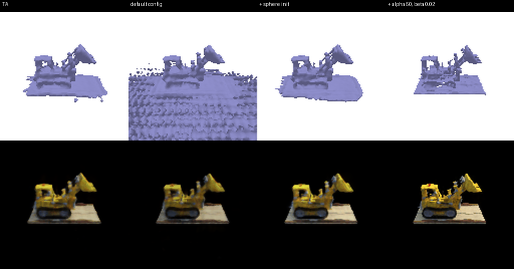
The TA's, default config, with sphere initialization, final
Beta from 0.1 to 0.01 (sphere initialization, alpha = 10)
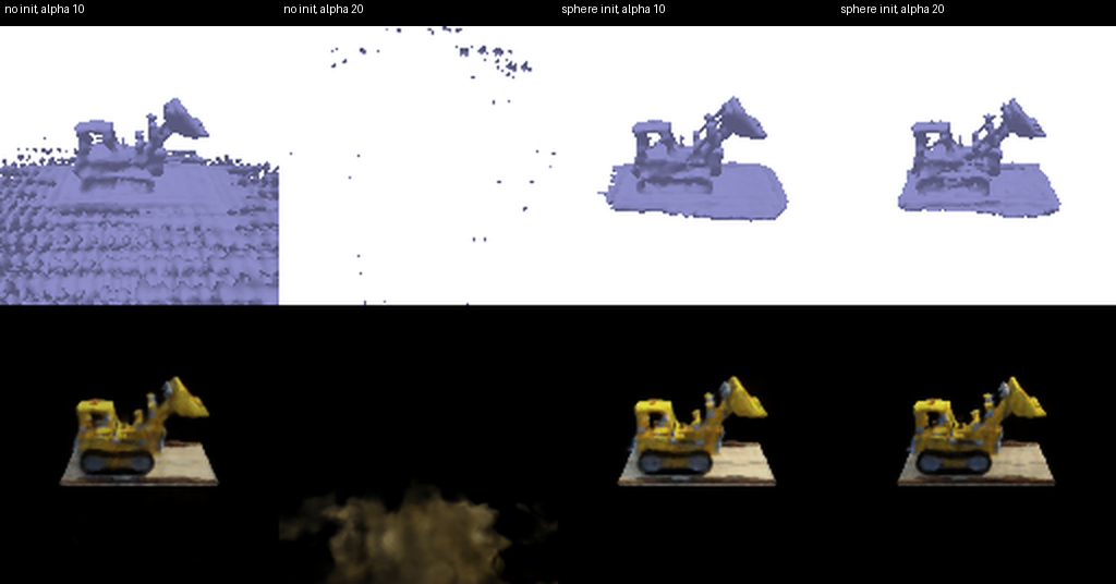
Alpha 10 and 20, without and with the sphere initialization
With the default config the colors look fine, but the mesh is covered in extra surfaces in the empty space around the bulldozer (522 pieces and 27x the area of my final mesh). The lego background is black, so a ray that hits nothing looks exactly like a ray that hits a black surface, and the color loss can't tell the difference. The network starts with a distance close to 0 everywhere, so it starts with zero crossings everywhere, and the ones the images don't see never get removed. A bigger eikonal weight doesn't fix it either, because a field with extra zero crossings can still have a gradient of length 1. So I used the geometric initialization from IDR and VolSDF, where the network starts out as the SDF of a sphere of radius 1 (the last layer is set so d(x) is about |x| - 1, and the weights on the sin and cos inputs start at 0). That way empty space starts out clearly outside the object and the network only has to carve the bulldozer out of the sphere. This one change got the mesh down to 11 pieces with 99.7% of the area in the bulldozer.
I also switched the ReLUs in the distance network to Softplus (with beta = 100 like IDR), which makes the SDF and its gradient smooth so the eikonal loss is smooth too. It helped a little (22.3 vs 22.1 dB) and made the base plate thinner and flatter.
The biggest PSNR gain came from setting alpha = 1 / beta like the VolSDF paper does. With alpha = 10 one sample inside the object only blocks 27% of the light, so the surface is see-through unless a ray goes through a few samples inside, and thin parts like the bucket and the arm can't become solid. With alpha = 50 one sample blocks 79%, so the thin parts render properly. Going from alpha = 10 to 50 (and beta from 0.05 to 0.02) brought the validation PSNR from 22.3 up to 24.1 dB.
A big alpha only works with the sphere initialization though. Without it alpha = 20 completely failed (13.0 dB): by the end of training the SDF was negative everywhere in the box (between -0.93 and -0.63), so all of space counts as inside and has density close to alpha. Every ray becomes solid within its first few samples, so the network can only paint blurry colors right in front of the camera. With the sphere initialization empty space starts outside the object where the density is low, and alpha = 20 does better than alpha = 10.
Alpha = 100 and beta = 0.01 actually had the best PSNR (24.3 dB), but 12% of its mesh area is floaters because a beta that small leaves the SDF unconstrained away from the surface (question 1), so I didn't think the extra 0.2 dB was worth it and kept alpha = 50, beta = 0.02. A bigger eikonal weight (0.1) didn't get rid of floaters and cost 0.4 dB. The final settings are in configs/volsdf_surface_best.yaml and can be trained with python -m volume_rendering_main --config-name=volsdf_surface_best.
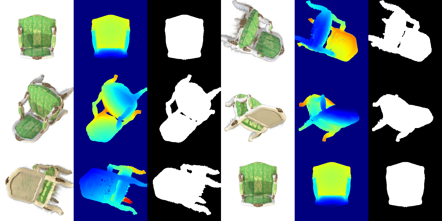
This is the pre-trained chair (283,873 Gaussians) rendered with my rasterizer by render.py, showing the color, depth and silhouette from 32 views. All 4 unit tests pass, and the frame that matches the reference image in the README is within 0.01 / 255 per pixel of it. Each frame takes about 16 seconds at 256 x 256 with 2048 Gaussians per splat.
The 3D covariance is R S S^T R^T from equation 6, where R comes from the quaternion (with quaternion_to_matrix) and S is a diagonal matrix of the scales. For isotropic Gaussians rotating a sphere doesn't do anything, so I skip the quaternion and just return s^2 times the identity. The 2D covariance is J W Sigma W^T J^T from equation 5, with J the Jacobian of the projection from _compute_jacobian and W the camera rotation. The 2D means are the 3D means projected to pixels with camera.transform_points_screen, and the power is -1/2 (x - mu)^T Sigma^-1 (x - mu) for every Gaussian and every pixel in one einsum. For sorting, the depth is the z coordinate of each mean in camera space, and I sort front to back with argsort and drop anything with negative depth since it is behind the camera. The alpha is opacity * exp(power), and the transmittance is a cumprod of (1 - alpha) over the sorted Gaussians, starting from the transmittance left over from the previous mini-batch. Then with weight = alpha * T, the color is the sum of weight * color, the depth is the sum of weight * z, and the silhouette is the sum of the weights (which is the total opacity). I didn't divide the depth by the silhouette, because render adds the mini-batches together and the sums only add up correctly that way.
I noticed two things in the starter code. First, it passed transmittance[-1] to the next mini-batch, which is the transmittance from before the last Gaussian in the batch, so that last Gaussian never blocked anything in later batches. I changed it to also multiply by (1 - alpha) of the last Gaussian. For this chair you can't see the difference, but now the result doesn't depend on the mini-batch size.
Second, unit test 2 (and test 4, which uses its covariances) expects W = camera.R. pytorch3d uses row vectors (x_cam = x_world R + T), so the rotation that acts on column vectors, which is what equation 5 needs, should be R^T. I checked this by sampling 400,000 points from one 3D Gaussian, projecting them with the camera and measuring the covariance of the projected points. W = R^T matches it to 3 digits ([3.70, -3.97; -3.97, 5.25] measured vs [3.69, -3.97; -3.97, 5.26]) and W = R doesn't ([2.23, 2.04; 2.04, 6.26]). The reference image in the README was made with W = R, since it matches my W = R render to 0.01 / 255 and my W = R^T render to only 1.96 / 255. I kept W = R in my code so the unit tests and the reference output match, but it means each splat's ellipse is rotated wrong, which shows up as fuzzy wisps around the edges.
Reference, W = R (submitted), W = R^T
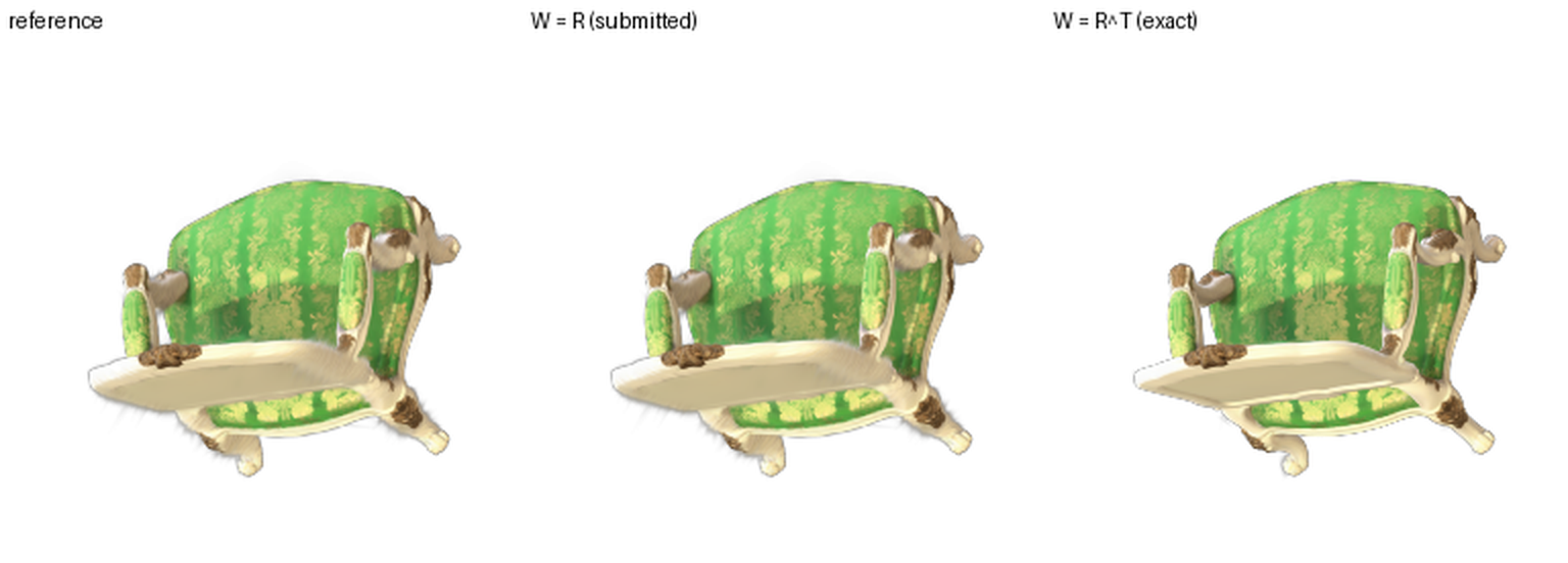
The wisps along the left edge of the seat and between the legs in the reference and in my W = R render go away with W = R^T, and the edges get sharper. About 2% of the pixels change by more than 30 / 255.
Mean PSNR = 30.52, mean SSIM = 0.946 on the 5 held-out views
Learning rates: opacities 0.05, scales 0.005, colours 0.02, means 0.002 (Adam)
Iterations: 3000
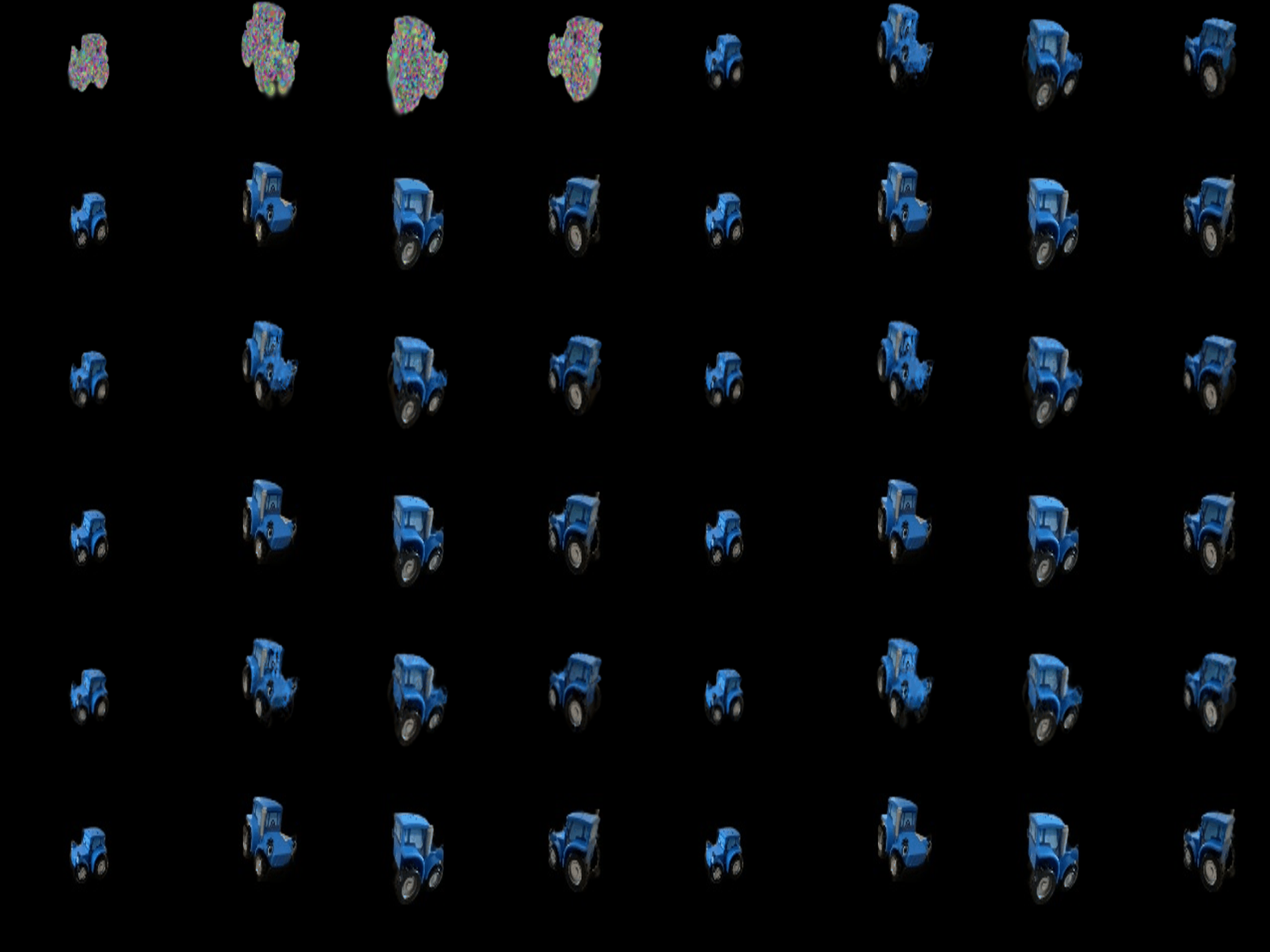
The top row is the Gaussians being trained, rendered every 60 iterations from 4 training views, and the bottom row is the ground truth.
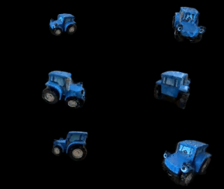
These are the renders of all 197 training views after training.
make_trainable turns on gradients for the means, scales, colours and opacities, and for the quaternions only when the Gaussians aren't isotropic, since rotating a sphere doesn't change it. setup_optimizer puts every group in one Adam optimizer with its own learning rate. Every step renders one random training view on a black background with scene.render and takes the L1 loss against the ground truth. The Gaussians start at the 10,000 points from the point cloud with random colors, opacity close to 1 and a scale equal to the average distance to their 50 nearest points. These Gaussians are spheres, so the W = R issue from part 5 doesn't matter here.
Choosing the learning rates
I started with a small learning rate for the means and bigger ones for the opacities and colors, like the original paper, and changed one group at a time. Everything is 1000 iterations except the last row.
| Opacities | Scales | Colours | Means | Iterations | PSNR | SSIM |
|---|---|---|---|---|---|---|
| 0.05 | 0.005 | 0.02 | 0.0005 | 1000 | 29.65 | 0.941 |
| 0.05 | 0.005 | 0.02 | 0.0001 | 1000 | 28.99 | 0.932 |
| 0.05 | 0.005 | 0.02 | 0.002 | 1000 | 30.12 | 0.943 |
| 0.05 | 0.005 | 0.02 | 0.005 | 1000 | 29.95 | 0.941 |
| 0.01 | 0.005 | 0.005 | 0.0005 | 1000 | 29.17 | 0.936 |
| 0.05 | 0.01 | 0.05 | 0.0005 | 1000 | 29.07 | 0.930 |
| 0.05 | 0.005 | 0.02 | 0.002 | 3000 | 30.52 | 0.946 |
The learning rate for the means mattered the most. The point cloud is only a rough starting point, so the Gaussians need to be able to move: going from 0.0001 to 0.002 gained 1.1 dB, and going up to 0.005 made it worse again, so 0.002 was the best one I tried. Changing the color, opacity and scale rates from where I started only made it worse. Training 3x longer with the best rates added another 0.4 dB, and the loss was still slowly going down at the end. I only ran each setting once and there are only 5 test views, so differences of a few tenths of a dB could just be noise, but the means learning rate and training longer clearly helped. The final rates are the defaults in train.py, and the result above is from python train.py --num_itrs 3000 --viz_freq 60.
With all spherical harmonics (Q7.1)
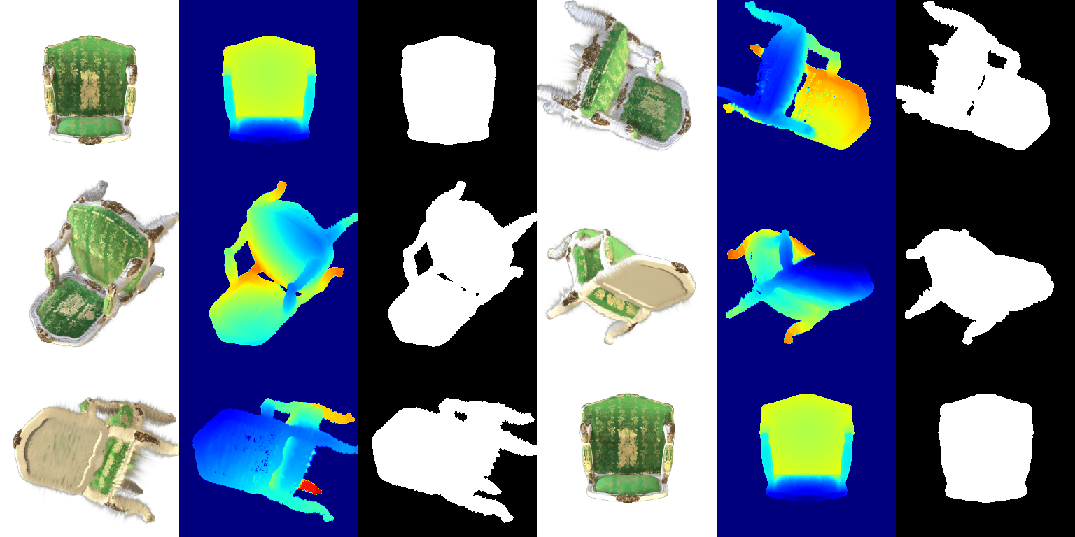
With only the DC color (Q5)
Each Gaussian has 48 spherical harmonic coefficients, 16 basis functions for each of the 3 color channels. calculate_gaussian_directions gives the unit vector from the camera center to each Gaussian, and colours_from_spherical_harmonics evaluates all 16 basis functions for that direction at once (a vectorized version of get_color from the linked implementation), takes the weighted sum of the coefficients, adds 0.5 and clamps at 0. render uses this color whenever the Gaussians have spherical harmonics, and render.py --dc_only turns it off, which gives exactly the same render as part 5. The frame of my render that matches the reference image with spherical harmonics is within 0.4 / 255 per pixel of it.
DC only (left), all spherical harmonics (middle), and their difference 4x brighter (right)

In frame 3, where we see the seat and the inside of the back from above, the green fabric is darker and more saturated with spherical harmonics and the gold pattern has more contrast, while with DC only the fabric looks lighter and flatter. The DC term is the color averaged over all viewing directions, so things like the sheen of the fabric get smeared into one in-between color. The white wood frame looks almost the same in both, so it doesn't change much with view.
Frame 14 has the back facing the camera and is one of the views with the biggest difference (7.9 / 255 on average). Head on, the gold threads in the middle of the backrest are a lot brighter with spherical harmonics and the green around them is darker, which looks like light reflecting off satin. The difference image is brightest over the whole backrest and seat and almost black on the frame and legs.
Frame 31 is the back from straight behind, and it shows the same thing: the gold motif in the middle is bright and the green is deep with spherical harmonics, and both are washed out with DC only. Over all 32 frames the average difference goes from 1.7 / 255 (frames 18 to 29) up to 7.9 / 255 (frame 14), so the view dependent effects are mostly on the fabric. Neither version gets rid of the white wisps around the edges of the chair, since those come from the shape of the Gaussians (part 5) and not their color.
Baseline: mean PSNR = 19.08, mean SSIM = 0.728
Improved: mean PSNR = 23.87, mean SSIM = 0.882
Baseline training progress
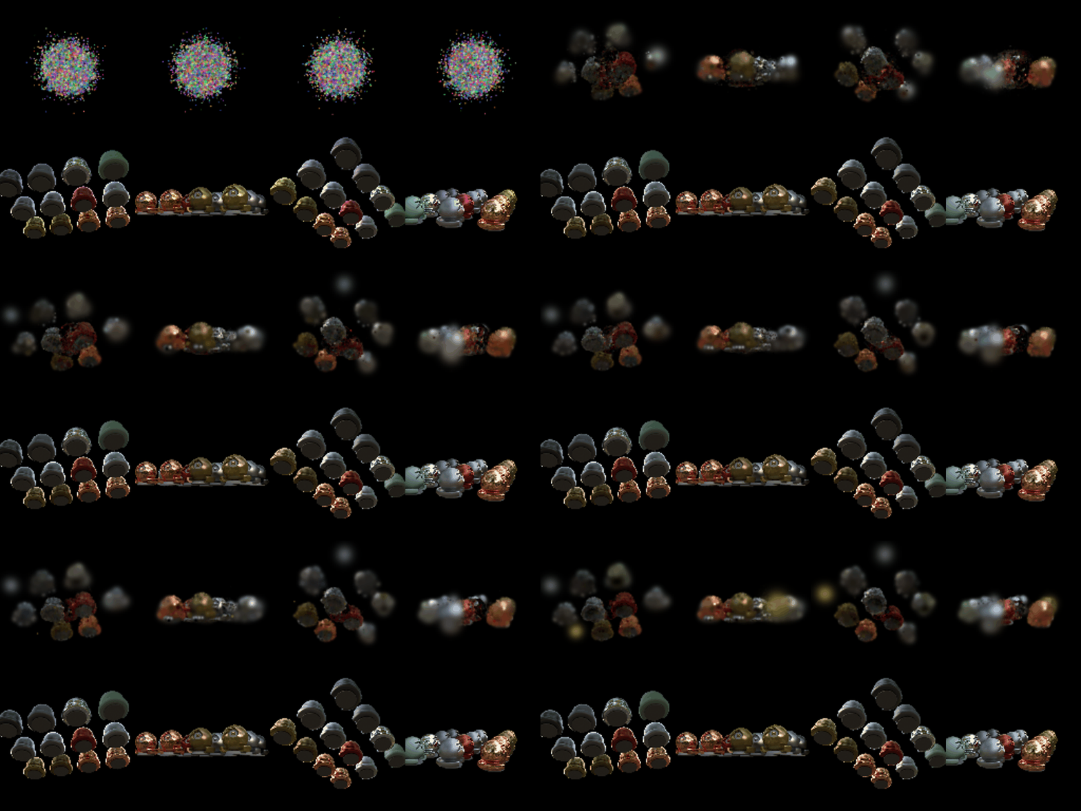
Improved training progress
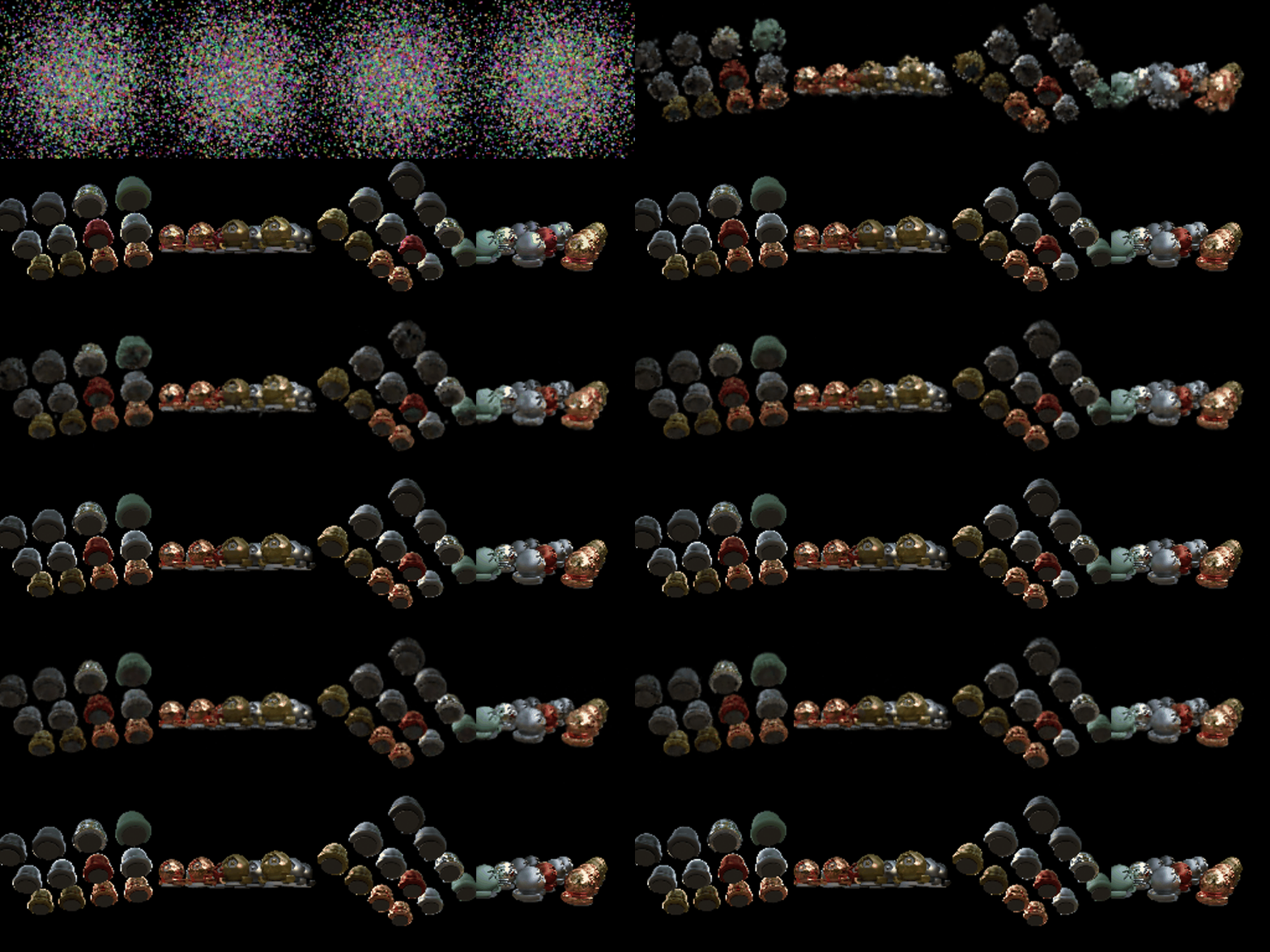
In both gifs the top row is the Gaussians being trained, rendered every 60 iterations from 4 training views, and the bottom row is the ground truth.
Final renders of the training views, baseline (left) and improved (right)
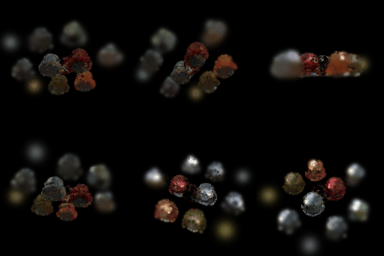
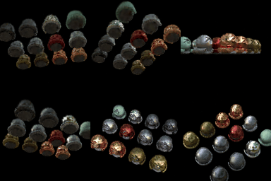
The baseline is exactly my setup from question 6 (isotropic Gaussians, the same learning rates, L1 loss, 3000 iterations) but starting from 10,000 random points with init_type="random". The PSNR and SSIM are on the 100 validation views of materials. In the baseline gif the spheres in the middle of the scene come in fine, but the ones on the outside stay blurry or never show up and just turn into faint glowing blobs. The random initialization puts all the points in a small ball (std 0.2) around the origin, while the materials spheres are spread over a much bigger area, so very few Gaussians ever reach the outer spheres and the baseline has no way to add more.
What I changed
To see what each change does, I added them one at a time and trained each version for the same 3000 iterations as the baseline.
| Version | PSNR | SSIM | Final number of Gaussians |
|---|---|---|---|
| Baseline (question 6 setup) | 19.08 | 0.728 | 10,000 |
| + wider initialization | 22.80 | 0.837 | 10,000 |
| + anisotropic Gaussians | 23.13 | 0.847 | 10,000 |
| + SSIM loss and learning rate decay for the means | 23.24 | 0.858 | 10,000 |
| + densification and pruning (final) | 23.87 | 0.882 | 18,213 |
Last frame of each version's training progress gif
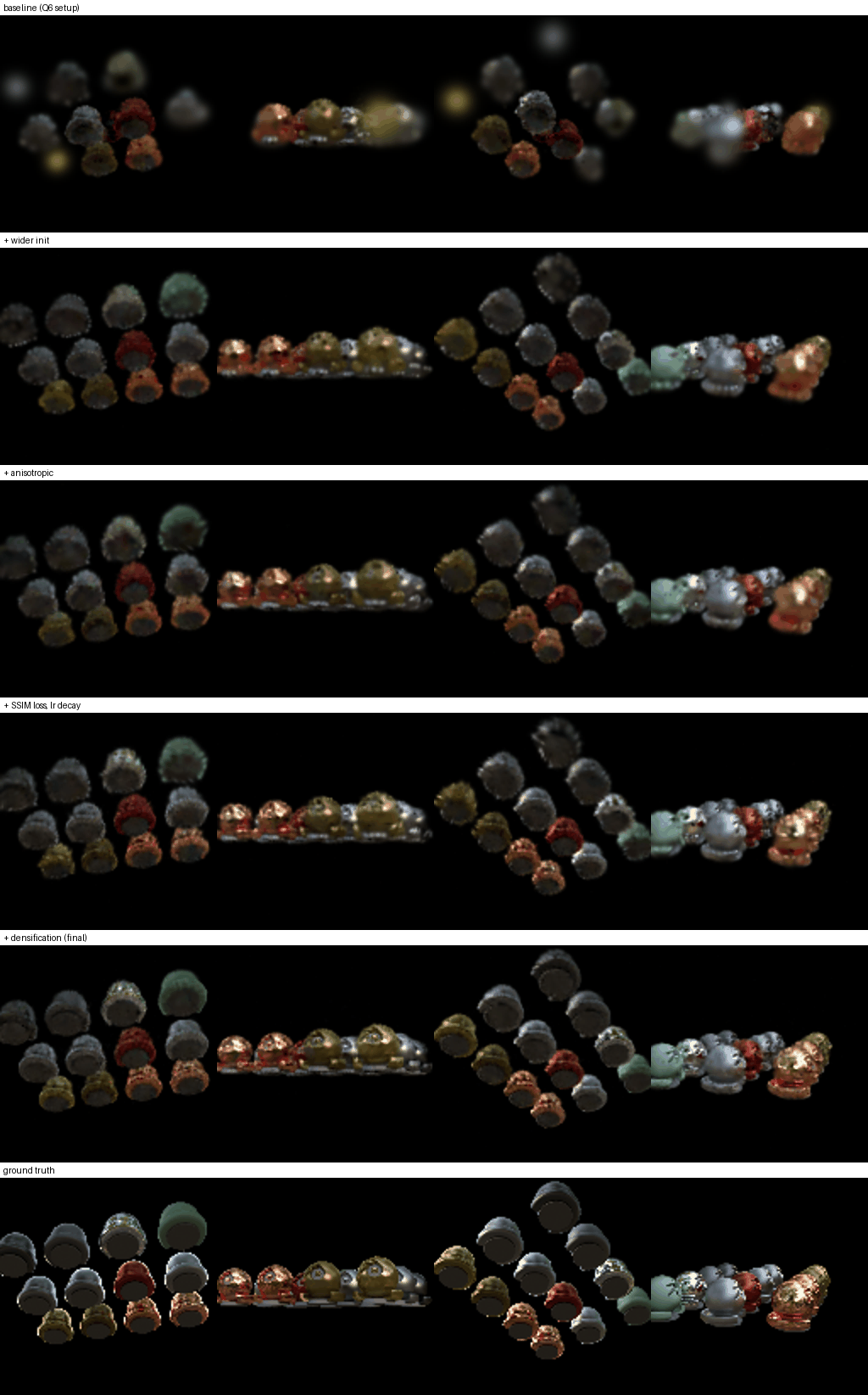
The first and biggest change was the initialization. Instead of the default std of 0.2, I spread the random means out with a std of 0.7 so they cover the whole area where the spheres are. This alone gained 3.7 dB, and now all 12 spheres show up, but they are fuzzy with spiky outlines because round isotropic Gaussians can't line up with the edges.
Next I switched to anisotropic Gaussians, so each one also learns a rotation and a different scale along each axis (the quaternions get a learning rate of 0.001). They can stretch along the surface of a sphere instead of sticking out of it, which makes the outlines smoother and gained 0.3 dB.
Then I changed the loss to 0.8 L1 + 0.2 (1 - SSIM) like the original paper, with an 11 x 11 Gaussian window for the SSIM, and made the learning rate of the means decay exponentially from 0.005 to 0.00005 over training (also like the paper). The higher starting rate lets the means move a lot early on, and the decay lets them settle at the end instead of jittering around. This mostly helped SSIM (0.847 to 0.858) and made the patterns on the spheres a bit sharper.
The last change was a simplified version of the paper's adaptive density control. During training I keep track of the average gradient of each Gaussian's mean, and every 300 iterations between iteration 500 and 2400 I take the 10% of Gaussians with the biggest gradients, since those are the places the current Gaussians can't explain. Small ones get cloned and big ones (biggest scale over 0.02) get split into two Gaussians that are 1.6x smaller and sampled from inside the original. I also remove any Gaussian with opacity under 0.005, and I cap the total at 25,000. Because the parameters are new tensors after this, I restart the Adam optimizer each time, which is simpler than the paper's version that copies the optimizer state over. The number of Gaussians grew from 10,000 to 18,213, mostly by cloning, and this gave another 0.6 dB and the best SSIM. In the figure above the reflections on the metal spheres and the dark bases under the spheres come out closest to the ground truth with this version.
More Gaussians also need more GPU memory, since the rasterizer computes every Gaussian at every pixel and keeps all of it for the backward pass (question 6 already used about 15 GB for 10,000 Gaussians at 160 x 90). To fit up to 25,000 I wrapped each mini-batch splat in torch.utils.checkpoint, so it gets recomputed during the backward pass instead of stored. This doesn't change the result, only the memory and speed.
I also tried the anisotropic version with W = R^T from part 5 instead of W = R. It got 23.19 dB / 0.852 vs 23.13 dB / 0.847, which is too small of a difference to mean much, so I kept W = R everywhere to match the rest of my code.
Everything is in train_harder_scene.py, and the defaults are still the baseline. The final version is python train_harder_scene.py --num_itrs 3000 --viz_freq 60 --init_std 0.7 --anisotropic --ssim_weight 0.2 --lr_means 0.005 --lr_means_final 0.00005 --densify --densify_until 2400 --max_gaussians 25000 --checkpoint_splat --gaussians_per_splat 4096.