All models were trained on a GPU with raw images. I did not use the --load_feat argument. Unless stated otherwise, every model was trained for 10,000 iterations with batch size 32 and learning rate 4e-4, and the F1 scores come from eval_model.py on the 678 chairs of the test set.
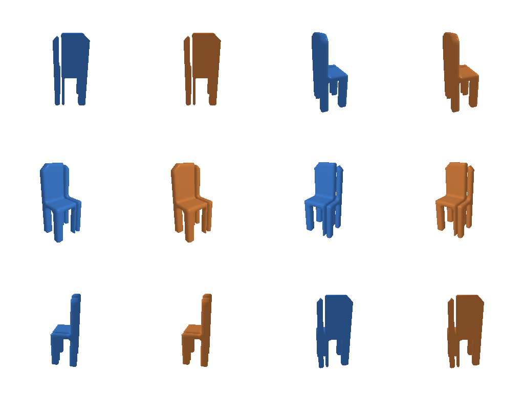
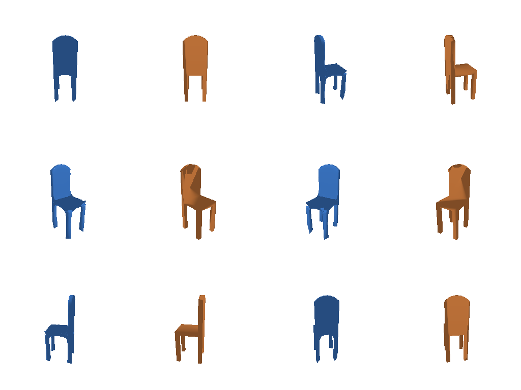
Left (blue) is the optimized voxel grid and right (orange) is the ground truth voxel grid. The loss is binary cross entropy with logits, so the grid being optimized holds unnormalized occupancy scores and I apply a sigmoid before rendering. The voxels are turned into a mesh with marching cubes at 0.5.
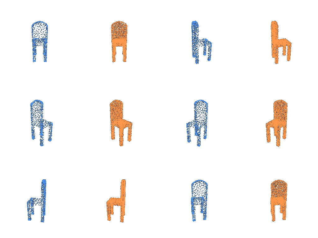
Left (blue) is the optimized point cloud and right (orange) is the ground truth point cloud. The chamfer loss is written from scratch with knn_points: for every point I find the squared distance to its nearest neighbour in the other cloud, average it in both directions and add the two terms. It matches the value of pytorch3d's chamfer_distance exactly.
Left (blue) is the deformed ico-sphere and right (orange) is the ground truth mesh. The smoothness loss is the uniform Laplacian smoothing loss, which pulls each vertex towards the average of its neighbours.
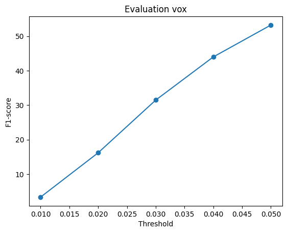
F1@0.05 = 53.2
Each example shows the input RGB, the predicted voxel grid and the ground truth mesh, followed by a 360 view of the prediction (blue) next to the ground truth (orange).
Test example 0 (F1@0.05 = 84.3)
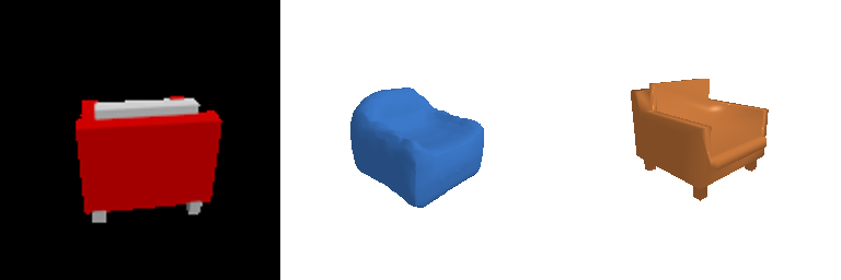

Test example 500 (F1@0.05 = 53.4)


Test example 600 (F1@0.05 = 89.2)

The decoder maps the 512-d ResNet18 feature with a linear layer to a 256 x 4 x 4 x 4 volume, then three transposed 3D convolutions (each followed by BatchNorm and ReLU) upsample it to 32 x 32 x 32, and a final 1 x 1 x 1 convolution gives one occupancy logit per voxel. Bulky chairs come out well, but thin parts like legs tend to disappear. Empty voxels make up most of each grid, so plain BCE lets the model win by predicting "empty" when it is unsure. 51 of the 678 test chairs came out completely empty, and these are scored as F1 = 0.
F1@0.05 = 78.9
Test example 100 (F1@0.05 = 92.5)
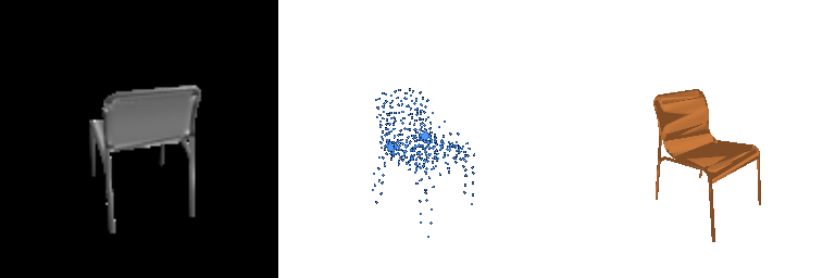
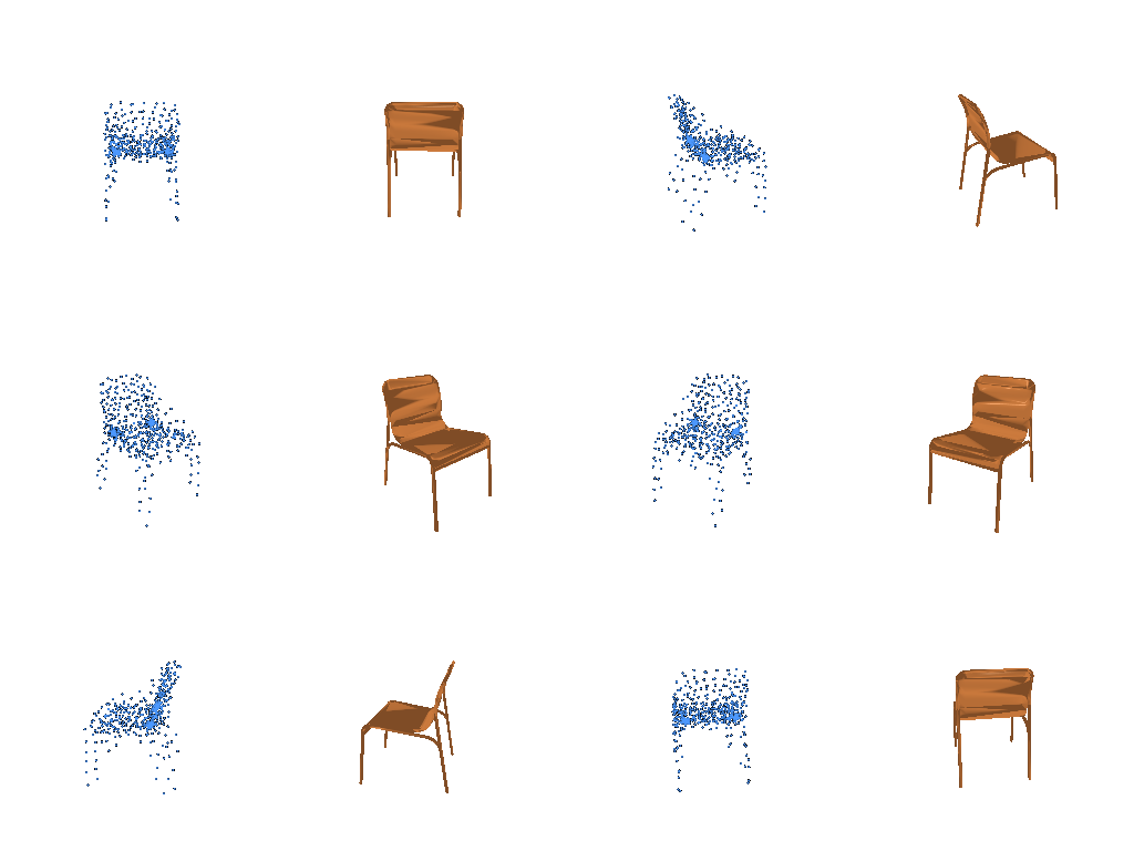
Test example 400 (F1@0.05 = 94.2)
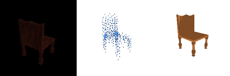
Test example 600 (F1@0.05 = 96.7)
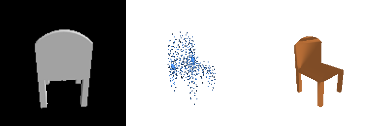
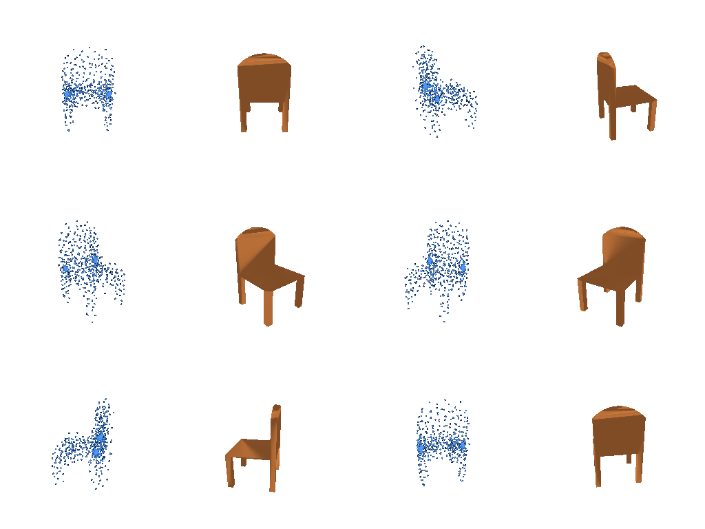
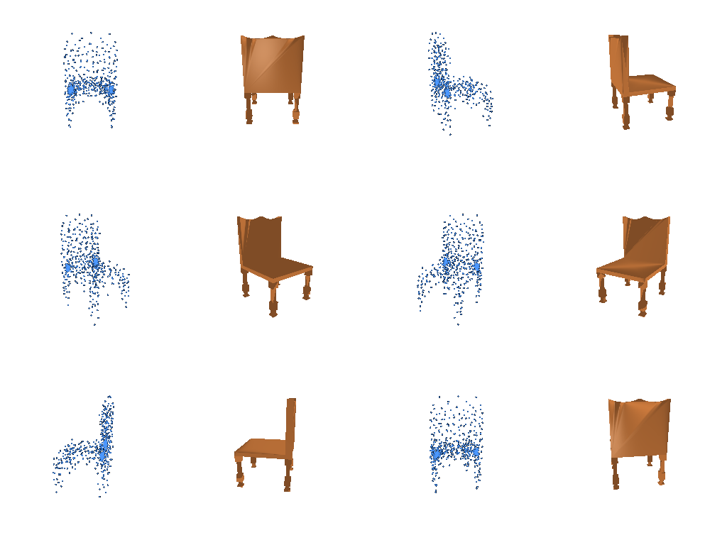
The decoder is an MLP (512 → 1024 → 2048 → 1000 x 3) that regresses all 1000 points at once. The predictions get the overall size and the back / seat / legs layout right, but they are fuzzy and look more like a generic chair than the specific one in the image. Many predictions also have a couple of dense clumps where several points collapse onto the same spot.
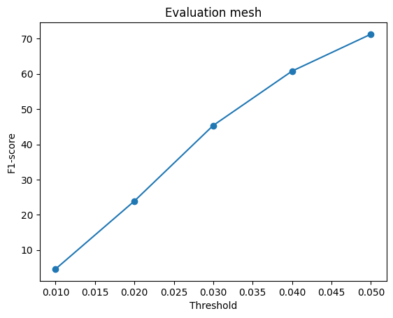
F1@0.05 = 71.3
Test example 200 (F1@0.05 = 84.1)
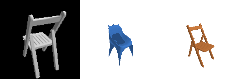
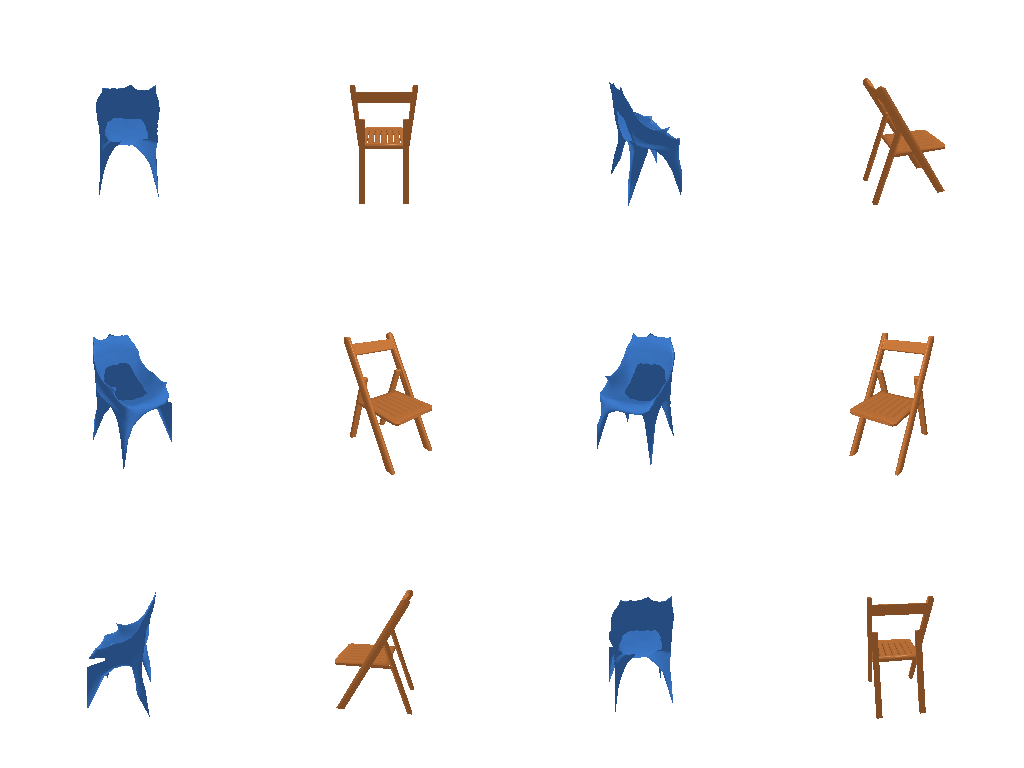
Test example 500 (F1@0.05 = 80.2)
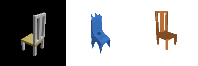
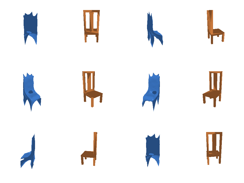
Test example 600 (F1@0.05 = 92.2)
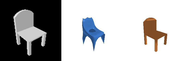
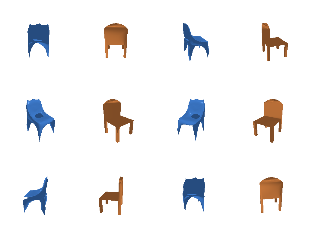
The decoder is an MLP (512 → 1024 → 2048 → 2562 x 3) that predicts an offset for every vertex of a level 4 ico-sphere. The last layer is initialized to zero so training starts from the clean sphere. I trained with --w_smooth 1.0 --n_points 5000, because the default w_smooth of 0.1 gave meshes that folded through themselves (see 2.4). The predictions are clean closed surfaces, but the legs come out as webbed fins and most seats have a dimple.
Comparing voxels, point clouds and meshes
| Representation | F1@0.05 | Median F1@0.05 | Chairs with F1 < 30 | Chairs with F1 ≥ 80 |
|---|---|---|---|---|
| Point cloud | 78.9 | 85.8 | 26 | 419 |
| Mesh | 71.3 | 74.3 | 14 | 263 |
| Voxel grid | 53.2 | 61.6 | 187 | 150 |
Point clouds score best because they are trained on exactly what the metric measures: F1 compares sampled surface points, and the point model is optimized with chamfer loss directly on its output points, where every point is free to go anywhere. The mesh is trained with the same chamfer loss but has to stay a deformed sphere. It is one closed surface with fixed connectivity, so it cannot open the gaps between legs or between back slats, and it webs across them. The smoothness term also trades some accuracy for a clean surface. In exchange, the mesh has the fewest bad failures, because a deformed sphere always gives a complete chair-shaped surface. Voxels are worst because of resolution and the loss. At 323 a chair leg is about one cell wide (even the ground truth voxels only reach about 78 F1@0.05 with this evaluation), and BCE dominated by empty space makes the model drop thin parts or predict nothing at all.
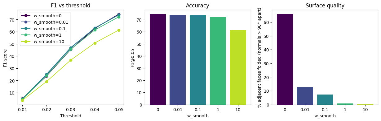
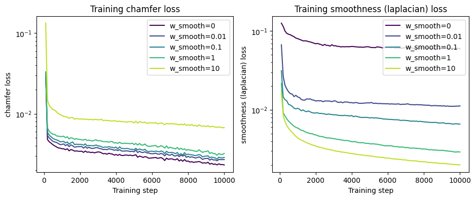
I varied w_smooth for the mesh model over 0, 0.01, 0.1, 1 and 10. To make it a controlled experiment, the five models were trained side by side on exactly the same batches, from the same initialization, with everything else fixed (5000 training points, 10,000 iterations). Besides F1, I measured how folded each surface is: the percentage of adjacent faces whose normals are more than 90° apart, meaning the surface doubles back on itself.
| w_smooth | F1@0.05 | Folded faces | Normal consistency (lower is smoother) | Laplacian (lower is smoother) |
|---|---|---|---|---|
| 0 | 74.5 | 65.8% | 1.259 | 0.0585 |
| 0.01 | 74.0 | 12.8% | 0.336 | 0.0111 |
| 0.1 | 73.8 | 7.4% | 0.216 | 0.0066 |
| 1 | 72.2 | 0.8% | 0.049 | 0.0029 |
| 10 | 61.4 | 0.1% | 0.021 | 0.0020 |
Test examples 0, 200 and 600. Columns: input, w_smooth = 0, 0.01, 0.1, 1, 10, ground truth.
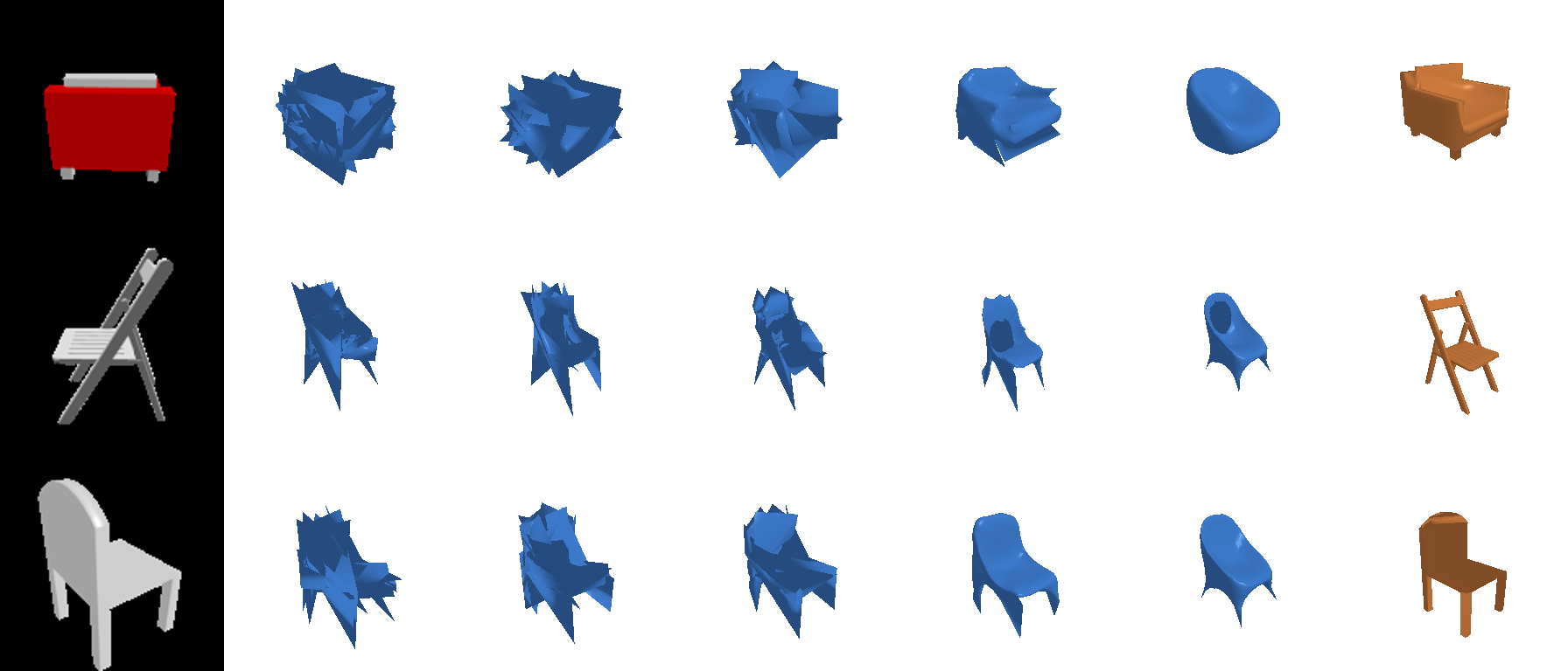

I made five visualizations of the trained mesh model (and the point model in one of them), each answering one question about what it learned.
Where does the mesh go wrong?
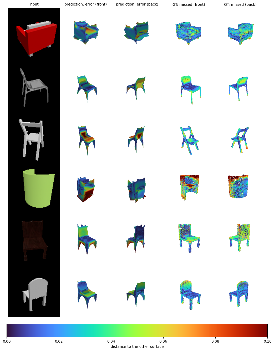
The predicted mesh is colored by its distance to the true surface (wrong geometry), and the ground truth is colored by its distance to the prediction (missed geometry). The model adds surface that isn't there in the seat dimple, in the webbing between the legs and on the barrel chair's bottom, and misses the extremities: leg tips, the barrel chair's top rim and the armchair cushions. It fills in between parts and drops their ends.
Error and variation over the whole test set
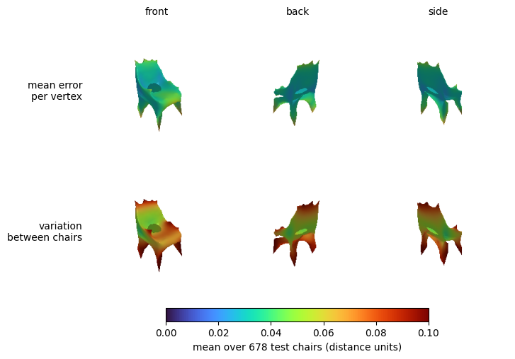
Every prediction deforms the same sphere, so vertex k means the same thing on every chair, and I can average per vertex over all 678 test chairs and paint the result on the mean predicted chair. The error is highest at the legs (0.036 in the bottom quarter vs about 0.031 elsewhere). The variation between chairs is also largest at the legs (0.068) and the top of the backrest, and smallest at the seat. The model keeps the seat as a fixed anchor and expresses differences between chairs mostly through leg spread and back height.
Learned correspondence
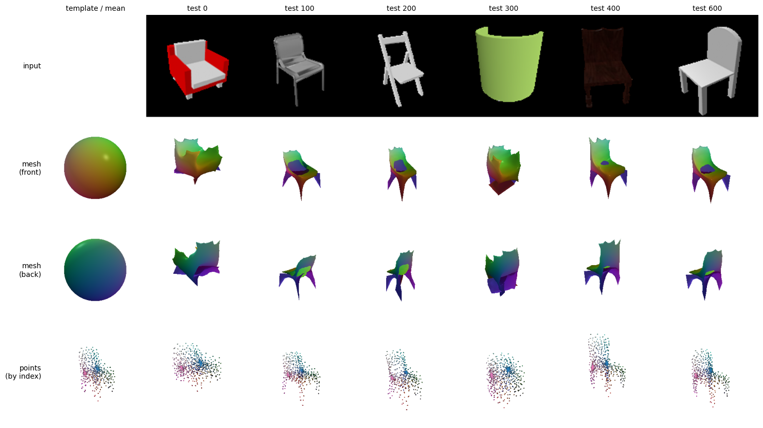
I colored the template sphere's vertices by their position and kept those colors on six very different predicted chairs. The same colors land on the same parts every time (green on the backrest top, purple on the legs, a blue patch at the seat), so the model learned a consistent mapping from regions of the sphere to chair parts without being told what a part is. The seat dimple from 2.3 is always the same blue patch of the sphere, which the model pinches inward because a closed sphere cannot open a hole. The point model (bottom row, colored by point index) also learned a consistent ordering, and its dense clumps are the same point indices on every chair.
Latent interpolation
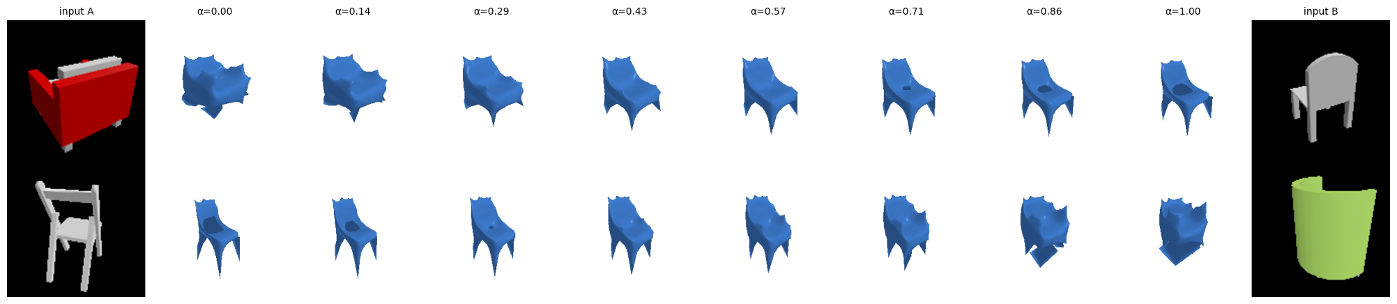

I blended the image features of two chairs and decoded the blends. Both morphs only pass through plausible chairs (from the armchair the bulk slims down and legs appear around α = 0.4), so the encoder learned a continuous space of chair shapes rather than memorizing examples. The jump near the end of the folding chair to barrel chair morph suggests that rare shapes like the barrel chair sit at the edge of that space.
Viewpoint robustness
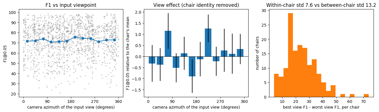
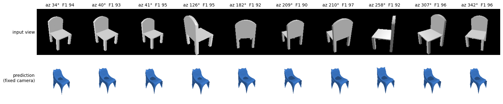
I evaluated 151 chairs from all 10 of their views (1510 predictions). After removing each chair's own mean, every 30° azimuth bin is within ±1.3 F1 of zero, so the model is about as good from the front, side or back. Which chair it is matters more than which view it gets (std between chairs 13.2 vs std across views of one chair 7.6). Chair 600 gets nearly the same 3D prediction (F1 90-97) from all ten views, including straight-on back and side views, so the model reconstructs the chair in a fixed object-centric frame and fills in hidden parts from a strong chair prior. Overall the model behaves like a template chair plus a few modes of variation (bulk, back height, leg spread), which makes it robust to viewpoint but is also why chair-specific details like separate thin legs are what it consistently gets wrong.
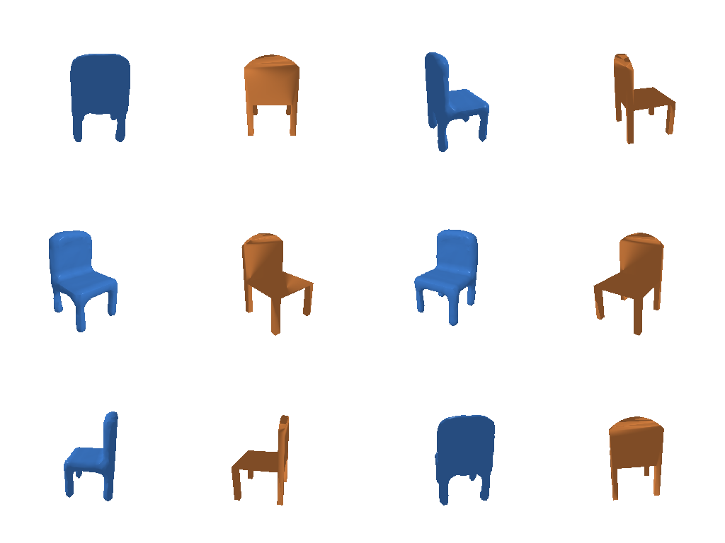
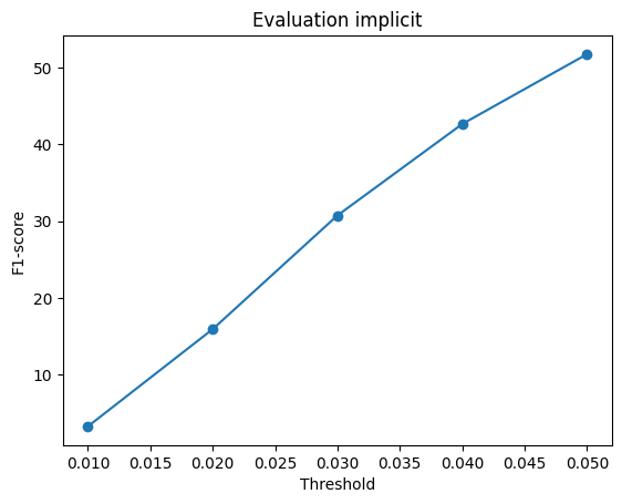
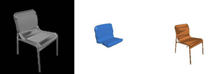
F1@0.05 = 51.7 (the voxel decoder in 2.1 gets 53.2)
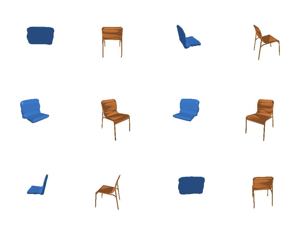
Test example 100 (F1@0.05 = 57.2, the voxel decoder gets 5.7)
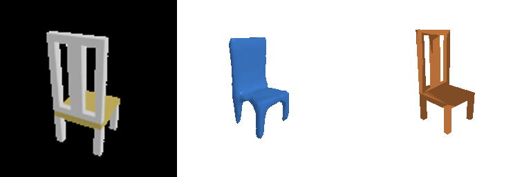
Test example 500 (F1@0.05 = 97.4)

Test example 600 (F1@0.05 = 90.0)
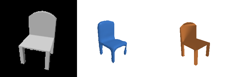
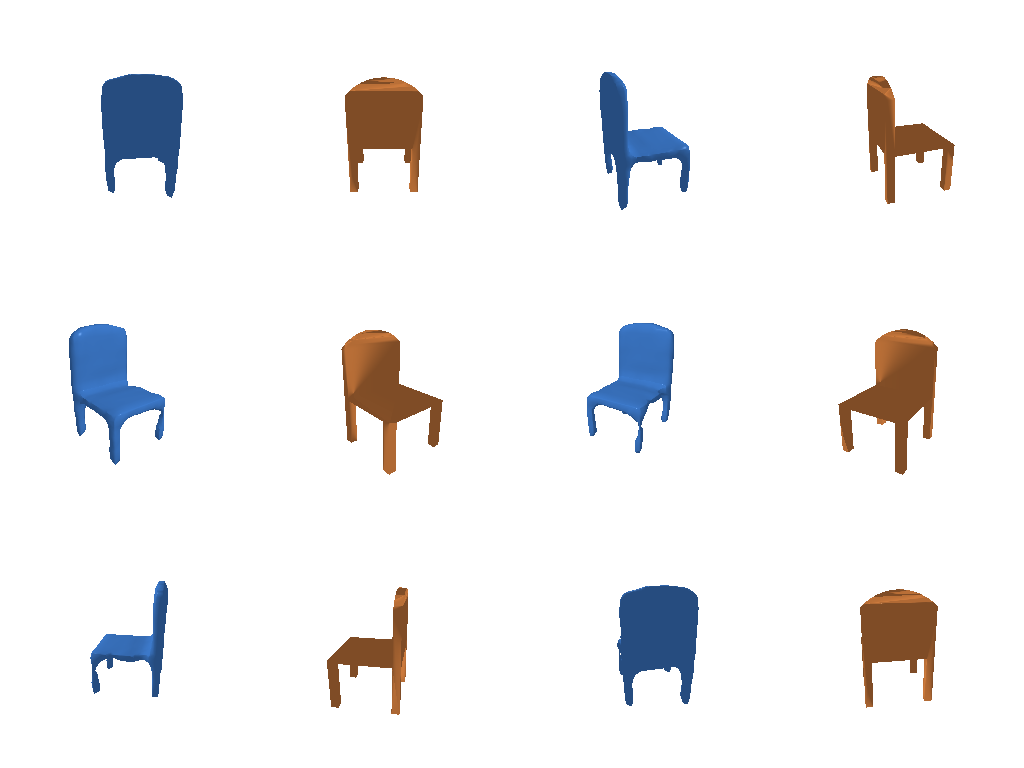
The implicit decoder is an occupancy network. An MLP takes a 3D query point in (-1, 1)3 and outputs an occupancy logit, with the image feature added at every layer (5 residual layers of width 128) and sin/cos positional encoding on the coordinates. For a prediction it is queried at all points of a 32 x 32 x 32 meshgrid, so it trains with the same BCE loss and is evaluated with the same marching cubes as the voxel decoder. The F1 is about the same as the voxel decoder (the 1.5 point gap is within run to run noise, since the evaluation picks random input views), with fewer empty predictions (42 vs 51) and smooth surfaces instead of blocky ones. It does this with about 0.4M parameters instead of about 11M. Both decoders hit the same limit, which comes from the 323 labels and the BCE imbalance rather than from the architecture.
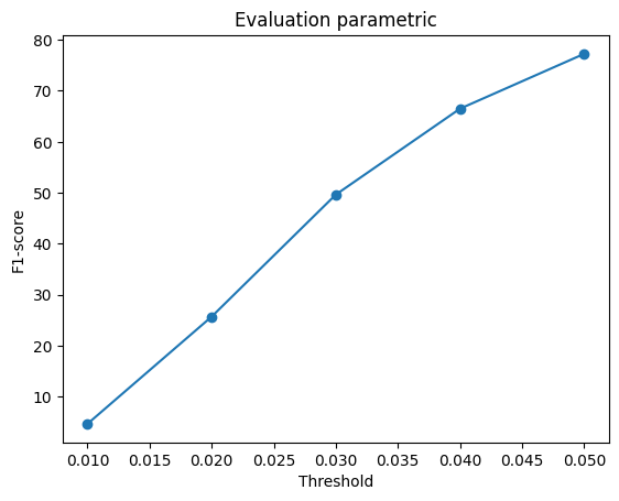
F1@0.05 = 77.2 (the point decoder in 2.2 gets 78.9)
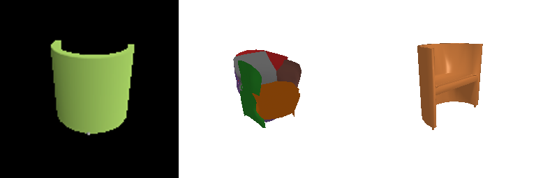
Each color is one patch.
Test example 300 (F1@0.05 = 70.5, the point decoder gets 58.4)
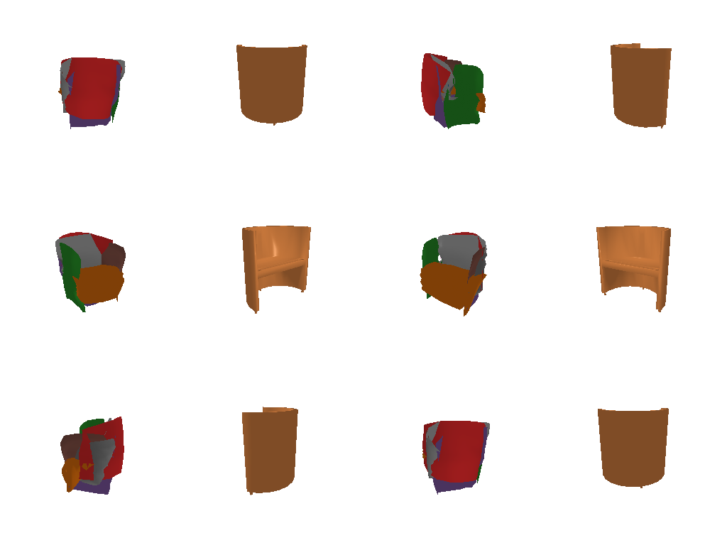
Test example 500 (F1@0.05 = 93.8)
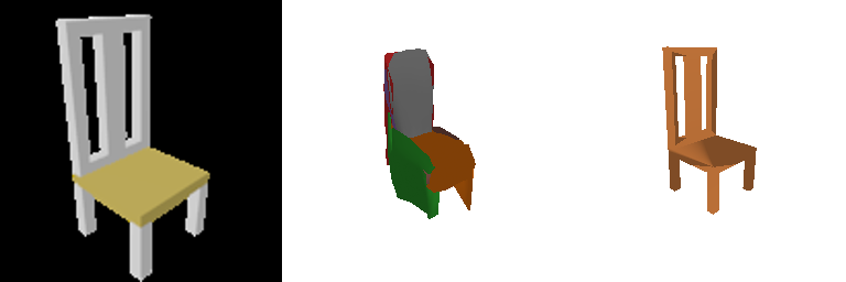
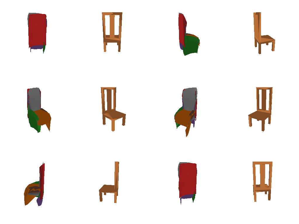
Test example 600 (F1@0.05 = 95.3)
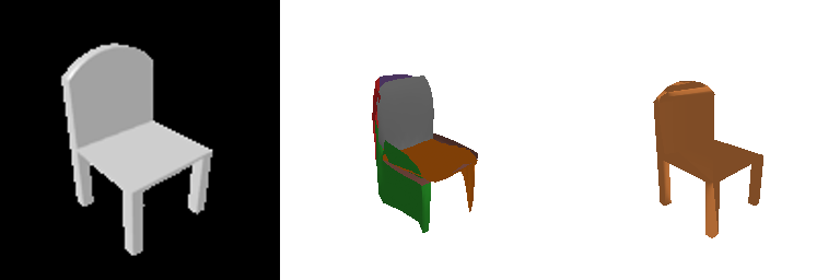
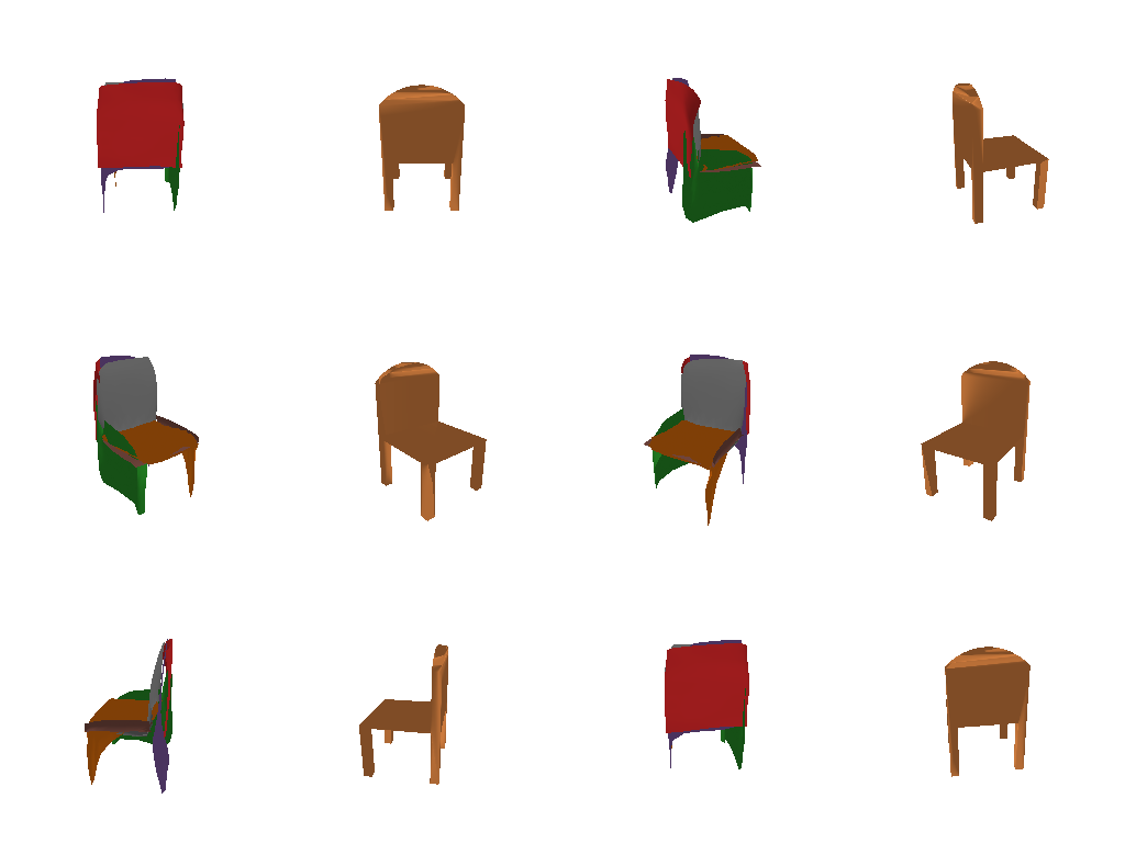
The parametric network follows AtlasNet. It has 8 patches, and each is an MLP that maps the image feature and a 2D point in [0, 1]2 to a 3D point. During training each patch gets new random 2D samples every step and the loss is chamfer. At test time each patch is sampled on a regular grid, so the output can be drawn as 8 surface sheets. It is 1.7 points below the point decoder with about 2.5x fewer parameters (3.4M vs 8.7M), better on bulky chairs and worse on thin ones. Each patch learned to cover the same part on every chair (gray for the back, orange for the seat, green for the front and legs), and the points are spread evenly along the patches without the clumps of the point decoder. Its weakness is that each patch is one smooth sheet, so 8 patches cannot form four separate legs and a back, and the legs get draped as panels.
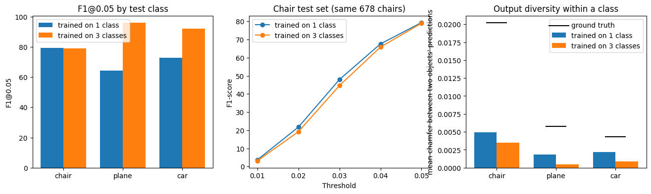
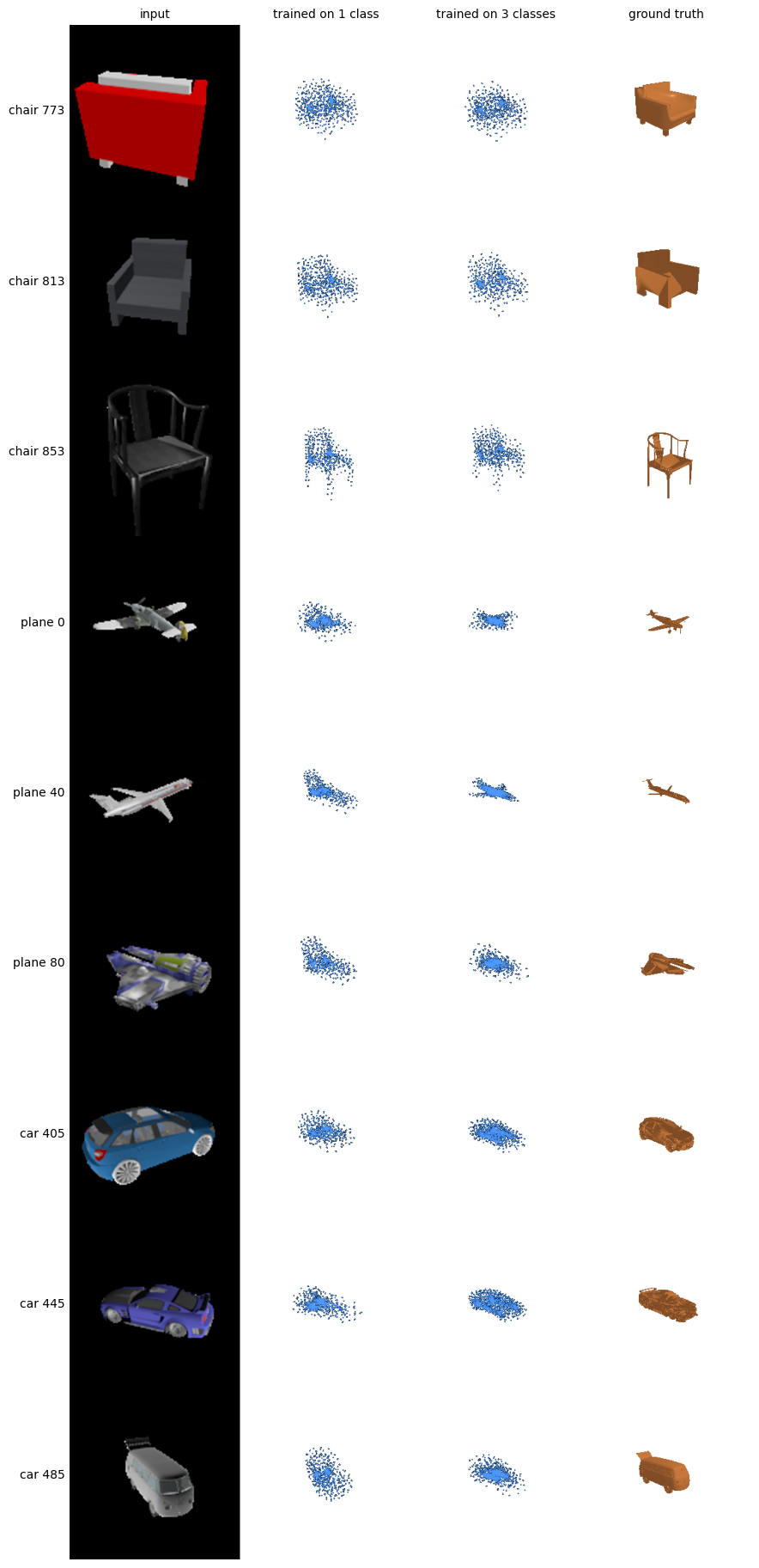
I trained the point cloud model on the three class dataset (chair, plane, car) with the same settings, and compared it with the chair-only model from 2.2 on the same test samples with the same input views. The chairs in the three class split are exactly the same 6100 training and 678 test chairs as in the chair-only split, plus 3640 planes and 3146 cars. Both models were trained for 10,000 iterations, so the three class model saw only about half as many chairs.
F1@0.05 of the three class model on the full three class test set: 87.1
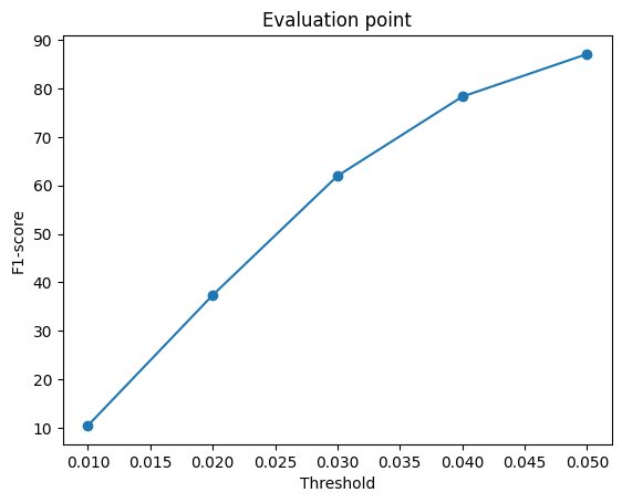
| Test class | F1@0.05, trained on 1 class | F1@0.05, trained on 3 classes | View consistency (1 → 3 classes, lower is more consistent) | Diversity (1 → 3 classes; ground truth) |
|---|---|---|---|---|
| Chair | 79.3 | 79.0 | 0.0012 → 0.0009 | 0.0050 → 0.0035; 0.020 |
| Plane | 64.2 | 95.9 | 0.0013 → 0.0002 | 0.0018 → 0.0005; 0.006 |
| Car | 72.8 | 92.1 | 0.0018 → 0.0005 | 0.0022 → 0.0009; 0.004 |
View consistency is the chamfer distance between the predictions for the same object from 3 different views. Diversity is the chamfer distance between the predictions for two different objects of the same class.