A.1. Differentiable Volume Rendering
1.1–1.2. Rendering pipeline
The camera defines a ray for each pixel. I sample points along each ray, evaluate density and color at those points, and combine the samples using their opacity and transmittance. The box is provided by the starter code; this part does not need training.
1.3. Ray sampling
I make a pixel grid in [-1, 1], unproject it into world space at camera depth 1, and subtract the camera center. I normalize the directions so the sample distances are in world units. The grid is flipped to match PyTorch3D's image coordinates.


1.4. Point sampling
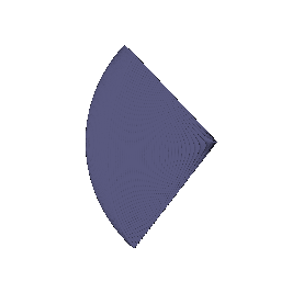
I use 64 evenly spaced distances from 0 to 5. Each sample is origin + distance × direction. Looking at all the samples from the first camera gives this cone-shaped point cloud.
1.5. Volume rendering
A sample's weight is its opacity multiplied by the light transmitted through the earlier samples. I use an exclusive cumulative product, so transmittance starts at 1.
alpha_i = 1 - exp(-density_i * delta_i)
T_i = product of (1 - alpha_j), for j < i
weight_i = T_i * alpha_i
color = sum_i weight_i * color_i
depth = sum_i weight_i * distance_i
The animation uses the default box settings and 20 cameras around the scene. The depth image is from camera index 2 and is divided by its maximum value. Empty rays have depth 0.


A.2. Optimizing a Basic Implicit Volume
2.1. Random ray sampling
I randomly choose 4,096 distinct pixels from each image and train on their rays. This keeps the backward pass smaller than rendering the whole image.
2.2. Loss and training
I use mean squared error between rendered RGB and the supplied images. I trained the box center and side lengths for 1,000 epochs over four views (4,000 updates), with Adam and a learning rate of 0.0005.
The fitted center is (0.25, 0.25, 0.00) and the side lengths are (2.01, 1.50, 1.50), rounded to two decimal places.
2.3. Visualization
The fitted box is wider along x than the initial cube. Its offset placement and soft boundaries look similar to the supplied reference.


A.3. Neural Radiance Field
I use six position-encoding frequencies and a six-layer, 128-wide MLP with a skip connection. A ReLU makes density nonnegative, and a small color head ends in a sigmoid. This model uses position only.
I trained on the 100 Lego training images at 128 × 128 for 250 epochs: 25,000 updates, with 1,024 rays and 128 samples per ray. Adam starts at 0.0005 and the learning rate decays by a factor of 0.8 every 50 epochs, using the supplied continuous schedule. Sampling is stratified during training and deterministic for evaluation.
The mean PSNR over all 100 validation views is 24.24 dB. The main shape is clear, but small studs and reflections are softer than in the ground truth. Here is the final 20-view spiral and one held-out view.


A.4.1. View Dependence
I add the encoded viewing direction to the color head. Density still depends only on position. The model shown uses four direction frequencies and 128 hidden color units.
I trained the materials models from scratch. All use the same 100 training views, 128 × 128 images, 25,000 updates, and the materials configuration's initial learning rate of 0.0001.
I also compared color-head capacity: two direction frequencies with 64 hidden units gave 24.01 dB on validation, while four frequencies with 128 units gave 24.24 dB. I selected the higher-validation-PSNR model for the figures below. Sharp reflections are still difficult at this resolution.
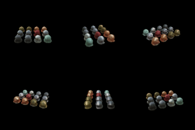

With the same 64-unit color-head width, adding direction changes mean validation PSNR by +0.61 dB. The selected model shown above changes it by +0.84 dB relative to the position-only baseline. Direction-dependent color can represent reflections that a position-only field has to average together. Giving direction too much capacity can also let the network memorize training views. Keeping it out of the density network avoids making geometry explicitly depend on the camera.


A.4.2. Coarse/Fine Sampling
I train two separate NeRF networks. The first evaluates 64 stratified points per ray. Its rendering weights define a probability distribution; I draw 128 additional samples using inverse-CDF sampling and detach the distribution from the coarse network's gradients. I merge and sort the old and new distances, then evaluate all 192 points with the fine network.
The loss is the sum of coarse and fine RGB MSE. Both networks start from scratch and train for the same 25,000 updates as the Lego baseline. The final color comes from the fine network.

The mean validation PSNR changes by +0.59 dB, and measured training time is 1.77× the baseline. This is an equal-update comparison, not an equal-compute comparison: the hierarchical model evaluates 64 + 192 points across two networks, versus 128 points in the baseline. More samples go near likely surfaces, but the extra network and sampling pass cost time.


A.4.3. VolSDF
I predict a signed distance and RGB color with a shared position-encoded MLP. The distance branch has six 128-wide layers with Softplus activations; the color head ends in a sigmoid. An initial sphere plus an unrestricted learned residual gives the network a starting surface. RGB training can change its shape.
I use the VolSDF density conversion, with negative distance inside the object:
density(d) = alpha * 0.5 * exp(-d / beta)          if d >= 0
             alpha * (1 - 0.5 * exp(d / beta))    if d < 0
loss = RGB MSE + 0.02 * mean((||gradient(SDF)|| - 1)^2)
The Eikonal term encourages distance gradients to have unit length. I sample 1,024 random points in [-4, 4]³ for this term at each update. The ray sampling and 128 × 128 Lego data are the same as the basic NeRF setup. Each run uses 250 epochs (25,000 updates), 1,024 rays per update, and 128 samples per ray.
The α=10, β=0.05 run reached 22.28 dB PSNR and 0.832 SSIM. The α=20, β=0.025 run reached 23.38 dB PSNR and 0.866 SSIM. I selected α=20, β=0.025 for the figures. Both settings keep αβ=0.5 while changing transition width. The learning rate starts at 0.0005 with the same decay as A.3. The gray-blue geometry is the extracted SDF zero level set, sampled on a 160³-cell grid in [-1.5, 1.5]³.
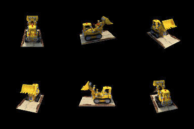

The tracks, body, and raised arm are recognizable in both views. The mesh still has rough patches and holes around thin parts, so a good color rendering does not mean the surface is fully recovered. The smaller beta gives a narrower density boundary, while keeping it large enough for the fixed ray samples to resolve.
Alpha, beta, and the learned surface
Alpha sets the interior density: larger values make a given thickness more opaque. Beta controls how gradually density changes across the surface.
High versus low beta: high beta spreads density outside the zero surface and tends to blur boundaries. The learned SDF may shift to compensate. Low beta makes density closer to a sharp inside/outside indicator.
Which is easier to train? A moderately high beta usually helps early training because gradients extend farther from the current surface. Very low beta concentrates them into a narrow region that ray samples can miss.
Which can give a more accurate surface? A lower beta can give tighter surface localization after convergence, provided sampling is dense enough. It is not automatically better: an excessively small beta with only 128 samples can make optimization and numerical integration unreliable.
Part A Evaluation
Scores in this table average the full 100-view validation split at 128 × 128. These views are separate from the 100 training views. I use RGB PSNR with pixel values in [0, 1] and SSIM with a data range of 1. The three comparison views are fixed at indices 0, 33, and 66. Training times exclude periodic rendering and evaluation; image times average five full-image renders after a warm-up on an RTX 4090. Concurrent runs can affect timing.
| Model | Updates | PSNR (dB) | SSIM | Train (min) | Render (ms/image) |
|---|---|---|---|---|---|
| Lego: position only | 25,000 | 24.24 | 0.884 | 4.8 | 45 |
| Lego: coarse/fine | 25,000 | 24.83 | 0.898 | 8.5 | 89 |
| Materials: position only | 25,000 | 23.40 | 0.849 | 4.5 | 45 |
| Materials: view, 2 frequencies | 25,000 | 24.01 | 0.859 | 4.7 | 52 |
| Materials: view, 4 frequencies | 25,000 | 24.24 | 0.869 | 4.9 | 54 |
| VolSDF: alpha 10, beta 0.05 | 25,000 | 22.28 | 0.832 | 7.0 | 52 |
| VolSDF: alpha 20, beta 0.025 | 25,000 | 23.38 | 0.866 | 6.7 | 52 |
B.5. 3D Gaussian Rasterization
I project each Gaussian's mean and covariance into the camera image, sort by depth, and blend front to back with opacity and transmittance. Color, depth, and silhouette use the same weights. The render keeps transmittance between Gaussian batches and adds the remaining background color once at the end.
This uses the supplied pretrained chair with 283,873 anisotropic Gaussians. I rendered 32 views at 256 × 256, processing 2,048 Gaussians per splat. This part does not train a model. The four supplied Gaussian tests pass.

B.6. Training 3D Gaussian Representations
6.1. Parameters and optimizer
I initialize 10,000 isotropic Gaussians from the supplied truck point cloud and optimize their means, log scales, opacity logits, and RGB colors. Initial scales are half the RMS distance to each point's three nearest other points. Isotropic Gaussians do not need learned rotations.
I use Adam with these learning rates:
| Parameter | Learning rate |
|---|---|
| Means | 0.0001 |
| Log scales | 0.02 |
| Opacity logits | 0.05 |
| Colors | 0.01 |
6.2. Training and results
I minimize RGB L1 loss for 2,000 updates, using one training view per update. There are 197 training views and 5 held-out test views, at the original 160 × 90 resolution. The random seed is 1.
Mean held-out PSNR is 30.26 dB and SSIM is 0.946. These scores use all five test views, RGB values in [0, 1], and a data range of 1.
The truck's shape and main colors are reconstructed, although the cab still has some grainy patches compared with the ground truth.


B.7.1. Rendering Using Spherical Harmonics
I evaluate the real spherical-harmonic basis through degree 3 using the normalized direction from the camera to each Gaussian. The supplied coefficients give 16 values per color channel. I add 0.5 to the evaluated color and clamp negative values to zero. The geometry and opacity stay fixed; no SH coefficients are trained here.
The polynomial normalization follows the original implementation's SH basis.
Both animations use the same camera trajectory and rasterization settings. The first uses only the DC coefficient; the second uses all coefficients.


In view 0, full SH makes the green upholstery darker and gives the gold pattern more contrast. The DC-only seat looks more washed out.


In view 10, the tilted seat and back again have stronger green/gold contrast with SH. The stretched splats near the legs remain in both versions because their geometry is unchanged.


In view 20, the beige underside looks similar in both renders. The changes are smaller and mainly affect the remaining green upholstery and trim; SH does not remove the stray splats.