

Liza Dahiya
A. Neural Volume Rendering
All Part 1 results use configs/box.yaml: a 256×256 image, 64 samples per ray between depths 0 and 5, and a box SDF (side 1.75) converted to density with α = 1, β = 0.05.
Each pixel center is mapped to normalized device coordinates in [-1, 1], placed on the image plane at depth 1, and
unprojected to world space with camera.unproject_points(..., from_ndc=True). Rays start at the camera
center and point (normalized) through those image-plane points.
The stratified sampler places n_pts_per_ray evenly spaced depths between min_depth and
max_depth, and each sample point is origin + depth × direction.

For a ray with N samples at depths t1 < … < tN, with density σi and color ci at each sample:
_compute_weights computes Ti as an exclusive cumulative product of
(1 − αj + 10−10) along the ray, and _aggregate
takes the weighted sum, used for both color and depth.


Using configs/train_box.yaml, I optimized the box's center and side lengths (starting from center (0, 0, 0)
and sides 1.5) from four ground-truth images with known camera poses. Training used Adam (lr 5e-4) for 1,000 epochs.
Each iteration renders 4,096 rays rather than the full 256×256 image. I build the full pixel grid, shuffle it with
torch.randperm, and keep the first 4,096 pixels, so each pixel is picked at most once per batch.
The loss is the mean squared error between the rendered colors and the ground-truth colors at the sampled pixels. It fell to about 1e-6 by the end of training.
| x | y | z | |
|---|---|---|---|
| Box center | 0.25 | 0.25 | 0.00 |
| Box side lengths | 2.01 | 1.50 | 1.50 |


The NeRF maps a 3D position to density and color. It doesn't use the viewing direction. Settings follow
configs/nerf_lego.yaml:
The loss is MSE between rendered and ground-truth pixel colors. I trained for 250 epochs on 128×128 lego images with 1,024 rays per batch and 128 samples per ray between depths 2 and 6. I used Adam with lr 5e-4, decayed by 0.8 every 50 epochs. The mean loss per epoch fell from 0.088 in the first epoch to 0.0022 in the last, and PSNR on the 100 held-out validation views is 26.3 dB.


I did all three extensions. Every model trains for 250 epochs with the same schedule as Part 3. PSNR is the
average over the dataset's 100 training views and its 100 held-out validation views. The rendering is compared
against the ground truth sampled exactly as during training, since the starter's sample_images_at_xy
is offset by up to half a pixel from the raw image grid.
As in NeRF, density depends only on position, so geometry stays consistent across views. For color, the trunk's features pass through a linear layer and are concatenated with the encoded viewing direction (2 frequencies, 15 dimensions). A 64-unit layer then predicts RGB. I compared it with the position-only model from Part 3 on the materials scene, at both the 128×128 and 400×400 settings from the provided configs.
| Materials scene | Train PSNR | Val PSNR | Train − val gap |
|---|---|---|---|
| 128×128, position only | 24.79 | 24.64 | 0.15 |
| 128×128, view dependent | 25.84 | 25.65 | 0.19 |
| 400×400, position only | 23.95 | 23.82 | 0.13 |
| 400×400, view dependent | 24.99 | 24.83 | 0.16 |


The materials spheres are glossy and metallic, so their highlights move as the camera moves. A position-only model can't represent that: it averages the highlights from all training views into each point, which shows up as a speckled, blotchy texture. The view-dependent model renders smooth surfaces with coherent highlights, and it gains about 1 dB on held-out views at both resolutions.
Trade-off. More view dependence lets the network explain each training image with color alone. In the extreme, it can memorize each view's appearance and leave the geometry wrong, which then breaks on new views. The train−val gap grows slightly with view dependence here (0.15 → 0.19 dB and 0.13 → 0.16 dB), but held-out PSNR still improves clearly. Three choices keep this in check, all following NeRF:
Feeding direction in earlier or with more frequencies would fit the training views more closely but generalize worse.
Two separate NeRFs. The coarse network is evaluated at Nc stratified samples, jittered randomly within their bins during training. Its weights (detached) define a piecewise-constant PDF along each ray, and inverse transform sampling draws Nf more depths where the weights are large. The fine network is evaluated at all Nc + Nf sorted depths and produces the final color. Both networks are trained with the MSE loss. I compared it with uniform sampling on lego at two budgets. Times were measured alone on one H200 (1,024-ray training step; full 128×128 render).
| Lego | Points per ray (coarse + fine net) | Val PSNR | Train step | Render |
|---|---|---|---|---|
| Uniform 64 | 64 | 25.25 | 5.5 ms | 10.5 ms |
| Coarse 32 + fine 32 | 32 + 64 | 26.26 | 10.3 ms | 15.4 ms |
| Uniform 128 (Part 3) | 128 | 26.32 | 6.2 ms | 18.9 ms |
| Uniform 192 | 192 | 26.48 | 8.0 ms | 28.3 ms |
| Coarse 64 + fine 128 | 64 + 192 | 26.49 | 15.1 ms | 38.2 ms |


Quality. Coarse/fine sampling helps most when samples are scarce. With 64 points per ray for the fine network, it beats uniform 64 by 1.0 dB and matches uniform 128. It concentrates samples near surfaces instead of in empty space. At 128 or more uniform samples, a 128×128 lego image is already close to saturated, and coarse/fine gives about the same PSNR as uniform 192.
Speed. It costs a second network, a second forward/backward pass, and the sampling step. A training step takes about 2× as long as uniform sampling with the same number of fine-network points, and rendering about 1.5×. It also doubles the parameter count. So it is worth it when samples are the bottleneck (higher resolution, larger depth ranges, thin structures). It isn't worth it when uniform sampling is already dense.
What α and β do. α is the density inside the object: far inside, σ → α; exactly on the surface, σ = α/2; and outside, it decays to 0. β is how sharply density drops off across the surface. Density goes from about α to about 0 over a band a few β wide around the zero level set. As β → 0, this becomes a step function: a solid object with an infinitely thin surface.
| β (α = 10) | Train PSNR | Val PSNR |
|---|---|---|
| 0.02 | 24.14 | 23.93 |
| 0.05 | 24.19 | 23.96 |
| 0.1 | 23.85 | 23.64 |
| 0.3 | 22.33 | 22.16 |


Best result (β = 0.05, α = 10). β = 0.05 gave the best held-out PSNR, and β = 0.02 was within 0.03 dB. Both keep the thin arm and shovel attached and the tracks well defined. β = 0.05 is a good middle ground: it is narrow enough that the mesh matches the rendered surface, and wide enough that rays get gradient early in training. Two other choices also helped:


B. 3D Gaussian Splatting
A vectorized PyTorch rasterizer, used to render the provided pre-trained chair (283,873 Gaussians) from 32 views at 256×256, splatting 2,048 Gaussians per batch.
R (see the note below).camera.transform_points_screen.einsum.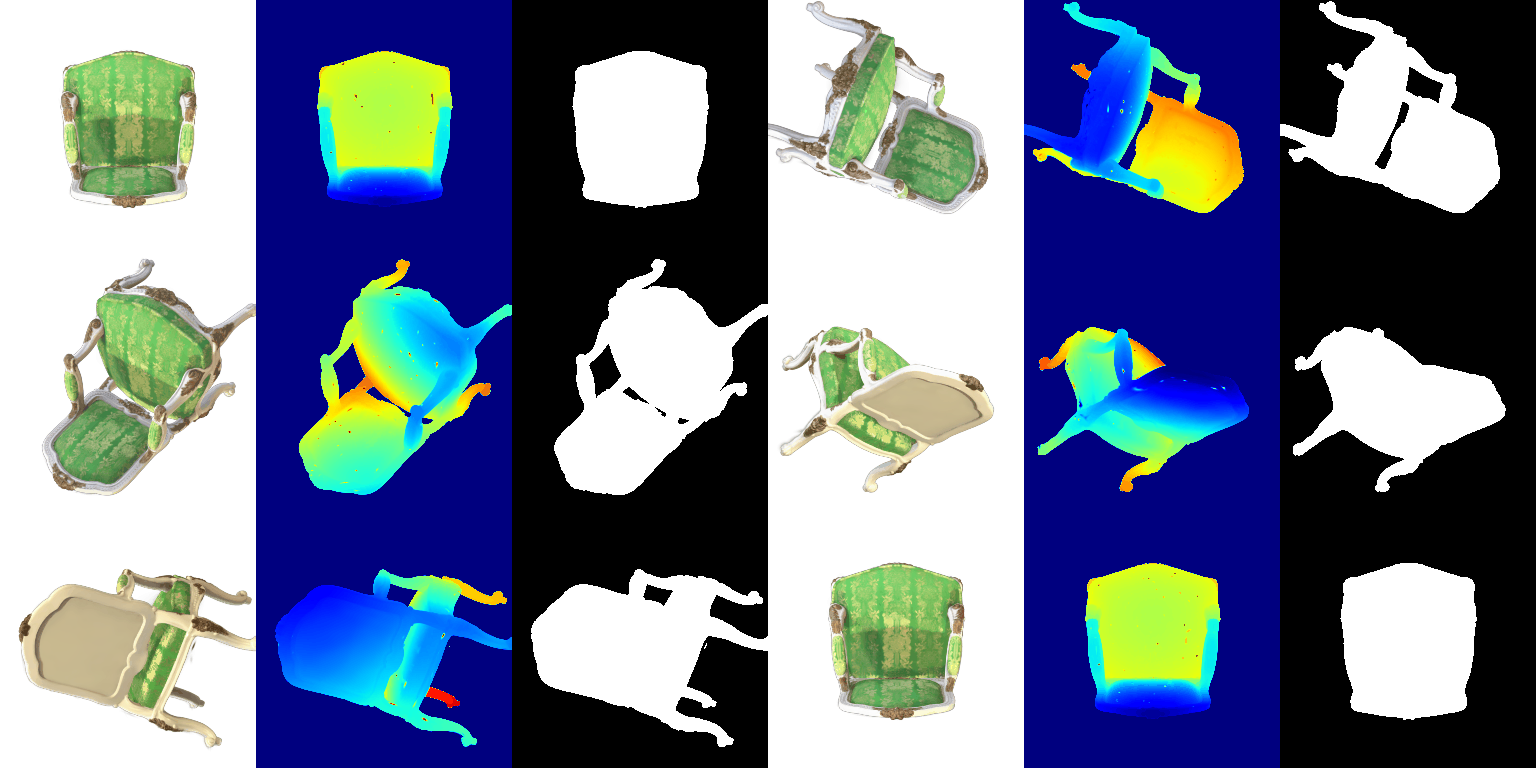
The provided unit tests and reference renders use W = R, PyTorch3D's rotation matrix as stored, and
the instructors allowed that convention on Piazza. I use W = RT for the final results, because it is
the one that matches PyTorch3D's projection. I rendered Part 5 both ways for comparison
(python render.py and python render.py --w_equals_r).
transform_points_screen) with autograd and formed Jtrue Σ
JtrueT. With W = RT the 2D covariance matches it to about 1e-7 relative error.
With W = R it is off by up to 75%.Gaussians.W_EQUALS_R = True, all 4 tests pass.| W = RT (final) | W = R (unit tests' convention) | |
|---|---|---|
| Unit tests passed | 2 / 4 (tests 2 and 4 fail) | 4 / 4 |
| Matches autograd Jacobian of the projection | yes (~1e-7) | no (up to 75% off) |

Same frames, W = RT (left) vs W = R (right):


With W = R, every splat's footprint is rotated by the wrong rotation. Elongated Gaussians get stretched in directions that don't follow the surface. The underside of the seat in frame 23 turns into a brushed, streaky texture, and spikes stick out of every edge: legs, armrests and frame. The same fringe is visible in the provided reference images. With W = RT, the seat underside is smooth and the silhouette is sharp. Both renders use the same Gaussians, so the difference comes entirely from the projection.
I also re-ran Parts 6 and 7 with W = R (the rest of the page shows the W = RT results):
| PSNR / SSIM | W = RT (final) | W = R |
|---|---|---|
| Q6 truck (isotropic) | 29.36 / 0.939 | 29.42 / 0.938 |
| Q7.2 baseline (isotropic) | 18.48 / 0.684 | 18.67 / 0.683 |
| Q7.2 improved (anisotropic) | 24.42 / 0.891 | 24.01 / 0.875 |
For isotropic Gaussians, Σ = s²I, so WΣWT = s²I for any rotation W, and the convention has no effect. The small Q6 and Q7.2 baseline differences are just run-to-run randomness. Only the anisotropic model depends on the convention. It does slightly better with W = RT (+0.4 dB, +0.016 SSIM). The gap is small because training is self-consistent either way: with W = R, the learned orientations partly adapt to the wrong projection.
The model uses 10,000 isotropic Gaussians, with means initialized from the provided truck point cloud. They are trained with the Part 5 rasterizer on the 197 training views, using an L1 loss between the rendered image (black background) and the ground truth. The optimizer is Adam with a separate learning rate for each parameter. Positions get the smallest rate: a small shift in a mean moves a Gaussian across pixels, while opacity and color can change quickly without destabilizing the scene.
| Parameter | Learning rate |
|---|---|
| Opacities (pre-sigmoid) | 0.05 |
| Scales (log) | 0.005 |
| Colours | 0.02 |
| Means | 0.0005 |
I trained for 1,000 iterations (one view per iteration). The L1 loss fell from 0.041 to 0.005. On the 5 held-out test views:
| Mean PSNR | Mean SSIM |
|---|---|
| 29.36 | 0.939 |


I did both extensions.
The pre-trained chair stores 16 spherical-harmonic coefficients per colour channel (degrees 0–3). Question 5 used only the degree-0 (DC) term, which is the same from every direction. For 7.1, each Gaussian's colour is computed from all 16 coefficients:
colours_from_spherical_harmonics evaluates the real SH basis up to degree 3 for all Gaussians at
once, then adds 0.5 and clamps at 0, the same post-processing as the DC colours.python render.py --use_sh renders with full SH. Without the flag, the question 5 render is
unchanged.
Side by side comparisons of the same frame, DC only (left) vs full SH (right). These are the three frames where the two renders differ most.

The upholstery is a darker, more saturated green with SH, and the gold floral pattern on the backrest stands out clearly. With DC only, the same fabric looks flat and washed out. The DC term is effectively the colour averaged over all viewing directions, so the sheen the fabric shows at some angles is spread evenly over every view and lightens it. The higher-order terms put that sheen back only where it appears from this viewpoint.

The DC-only render has a large pale-green patch across the lower middle of the backrest and lighter stripes between the motifs. That is sheen averaged in from other viewpoints. With SH, the same area is a deep, even green, and the gold motifs, especially the central one, become bright and metallic. Gold thread is specular, so it catches light only from some directions, and only the higher-order SH terms can represent that.

Seen from the front, the DC-only render again shows washed-out highlights in the middle of the backrest and on the seat cushion. With SH, those disappear, the fabric is darker and more saturated, and the central gold motif reads as shiny embroidery rather than a flat print. Geometry, silhouettes and depth maps are identical in both renders, since SH only changes colour. The difference is purely view-dependent appearance, and it matches the darker, more contrasted look of the TA's with-SH reference.
Both runs train 10,000 Gaussians from a random initialization on the 100 materials training views at
128×128 and are evaluated on the 100 validation views. train_harder_scene.py --method baseline and
--method improved reproduce them.
Isotropic Gaussians and init_type="random". The learning rates and L1 loss are the same as question 6
(opacities 0.05, scales 0.005, colours 0.02, means 0.0005), trained for 1,000 iterations.
| Mean PSNR | Mean SSIM | |
|---|---|---|
| Baseline | 18.48 | 0.684 |


The random initialization puts every Gaussian in a small ball (σ = 0.2) at the origin, but the spheres in this scene spread over roughly ±1.1 units. Starting there with a small learning rate, the Gaussians can't travel far enough in 1,000 steps. The central spheres are reconstructed as blurry clumps, and the outer ones appear only as faint blobs or not at all.
Same number of Gaussians (10,000), the same random-init entry point (init_type="random") and the same
data, trained for 3,000 iterations.
| Iterations | Mean PSNR | Mean SSIM | |
|---|---|---|---|
| Baseline (question 6 setup) | 1,000 | 18.48 | 0.684 |
| Improved | 3,000 | 24.42 | 0.891 |
| Parameter | Learning rate |
|---|---|
| Opacities (pre-sigmoid) | 0.05 |
| Scales (log) | 0.005 |
| Colours | 0.02 |
| Means | 0.002, decayed exponentially to 0.00002 by the last iteration |
| Quaternions | 0.002 |
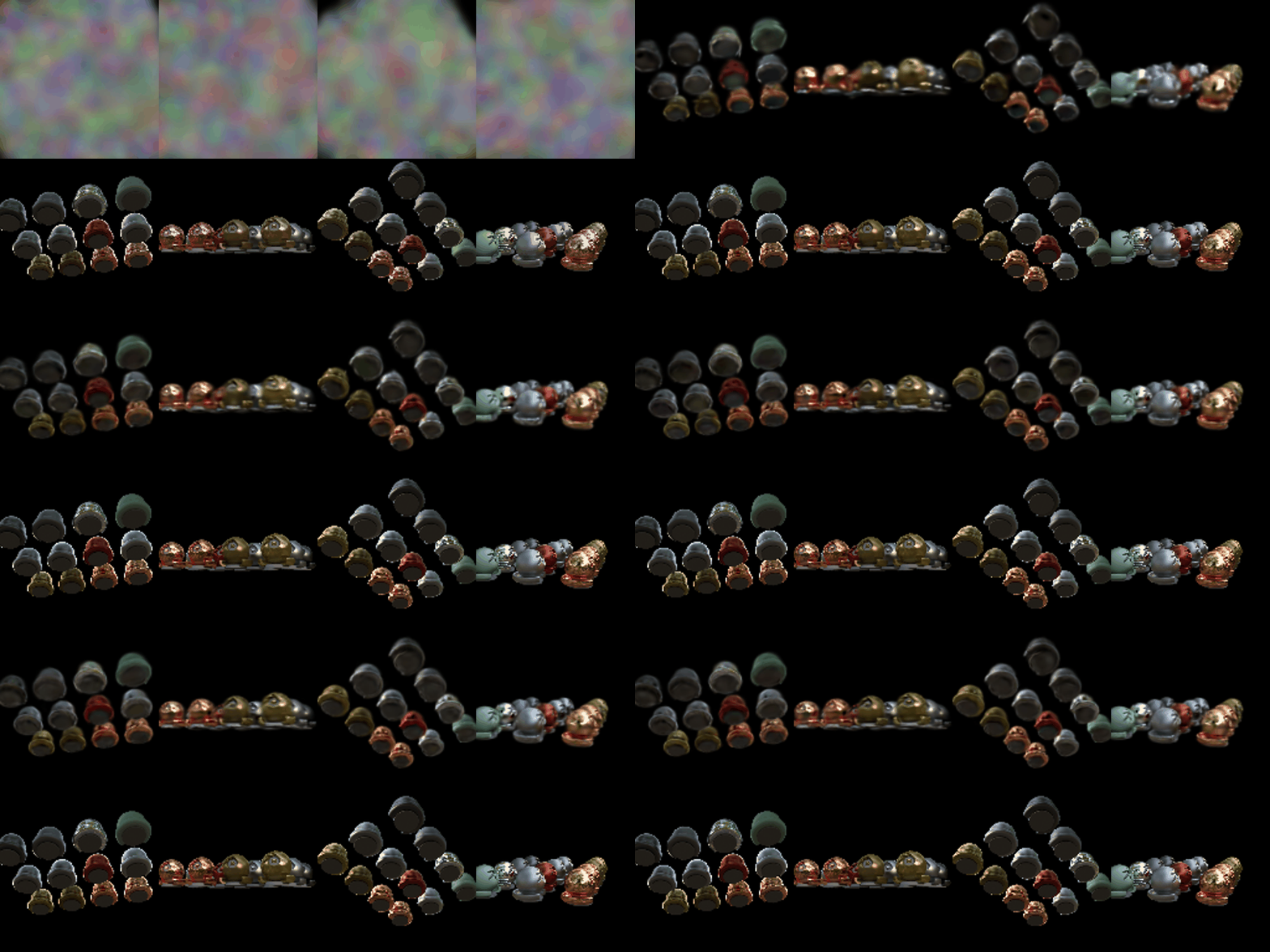

The improved model recovers all 13 spheres in the right places and colours. The baseline only produces blurry clumps near the centre. What's still missing is the sharp view-dependent detail: mirror and glass reflections come out as averaged colour, because these Gaussians have a single colour each, with no spherical harmonics.
Changes compared to question 6: