

16-825: Learning for 3D Vision · Kashu Yamazaki
Pixel centres are placed on a W×H grid spanning [−1, 1] in NDC. Each pixel
is lifted to depth 1 with camera.unproject_points; the ray origin is the camera
centre and the direction is the normalized vector from the origin to that point.
64 depths evenly spaced in [near, far] are shared by every ray: p = o + t·d.

Weights are wi = Ti(1 − e−σiΔti)
with Ti = ∏j<i e−σjΔtj
(an exclusive cumulative product, so T1 = 1). Colour and depth are the
weighted sums of per-sample colour and sample distance.


Training rays are a random subset (randperm) of the pixel grid, and the loss is the
MSE between rendered and ground-truth colours. After 1000 epochs:
| x | y | z | |
|---|---|---|---|
| Box centre | 0.25 | 0.25 | 0.00 |
| Side lengths | 2.01 | 1.50 | 1.50 |

The positional encoding uses 6 frequencies on xyz. A 6-layer, 128-unit ReLU MLP with the
encoding re-concatenated at layer 3 produces a feature; a linear head with ReLU gives density,
and a linear 128→128 layer followed by a 128→64→3 head with a sigmoid gives colour. Training follows
nerf_lego.yaml: 250 epochs of 1024 rays per image, 128 samples per ray, Adam at
lr 5e-4 decayed by 0.8 every 50 epochs, MSE loss. Test PSNR (200 held-out views,
128×128) is 24.09 (train 24.52).
Note on NeRF metrics. The provided training loop saves a checkpoint only every 50 epochs,
so the last saved model is from epoch 200. All PSNR values in A3 and A4 are computed from these
epoch-200 checkpoints with eval_nerf.py; the GIFs are rendered during training at
epoch 240.

The colour head additionally takes the harmonic embedding (2 frequencies) of the ray direction,
concatenated with the position feature. Density still depends on position only, as in NeRF, so
the geometry is shared across views and only the emitted colour can change with direction.
Same schedule as the lego run, at lr 1e-4 per nerf_materials.yaml.
| Materials | Train PSNR | Val PSNR | Test PSNR | Train − test |
|---|---|---|---|---|
| No view dependence, 128² | 23.47 | 23.35 | 23.03 | 0.44 |
| View dependence, 128² | 24.27 | 24.12 | 23.64 | 0.63 |
| View dependence, 400² | 24.40 | 24.26 | 23.79 | 0.61 |


View dependence lets the network represent the specular highlights of the metallic and glossy spheres, which a position-only colour can only average into a dull, view-independent tint; it raises test PSNR by 0.6 dB. The cost is a larger train–test gap (0.44 → 0.63 dB): with direction as an input the network can also explain a training pixel by a colour that is only correct from that particular view, instead of by better geometry. The design follows NeRF to limit this: density does not depend on direction, the direction uses only 2 frequencies, and it enters late, through a small head. I did not test variants with more direction capacity (direction fed to the density, or more frequencies); the expected risk is that the network memorizes the training views and produces wrong colours or floaters from new viewpoints. All numbers are from a single run each, so the 0.6 dB gain and the 0.2 dB change in the gap carry run-to-run noise.
Covariances are Σ = R S ST RT (or s2I
for isotropic Gaussians) and project as Σ' = J W Σ WT JT;
means are projected with transform_points_screen. Gaussians behind the camera are
dropped, the rest sorted by view-space depth, and colour, depth and mask are the
αT-weighted sums of colour, depth and 1.
Note on W. PyTorch3D stores R for row vectors
(xview = xworldR + T), so the world-to-view rotation in the
column-vector formula is W = RT. The provided unit tests 2 and 4 expect
W = R; with RT they fail while tests 1 and 3 pass. Projecting
200k samples of a 3D Gaussian through the camera gives an empirical 2D covariance that matches
W = RT to three decimals; with W = R one diagonal entry is
3.4× too large and the off-diagonal term has the wrong sign,
and with W = R the chair's anisotropic splats render as visibly mis-oriented
streaks. The renders below use RT.

| Parameter | Learning rate |
|---|---|
| Opacities (pre-sigmoid) | 0.05 |
| Scales (log) | 0.005 |
| Colours | 0.02 |
| Means | 0.0005 |
Adam, L1 loss, 1000 iterations, isotropic Gaussians initialized from the provided 10k-point cloud. On the 5 held-out test views of the truck dataset: PSNR 29.49, SSIM 0.939.
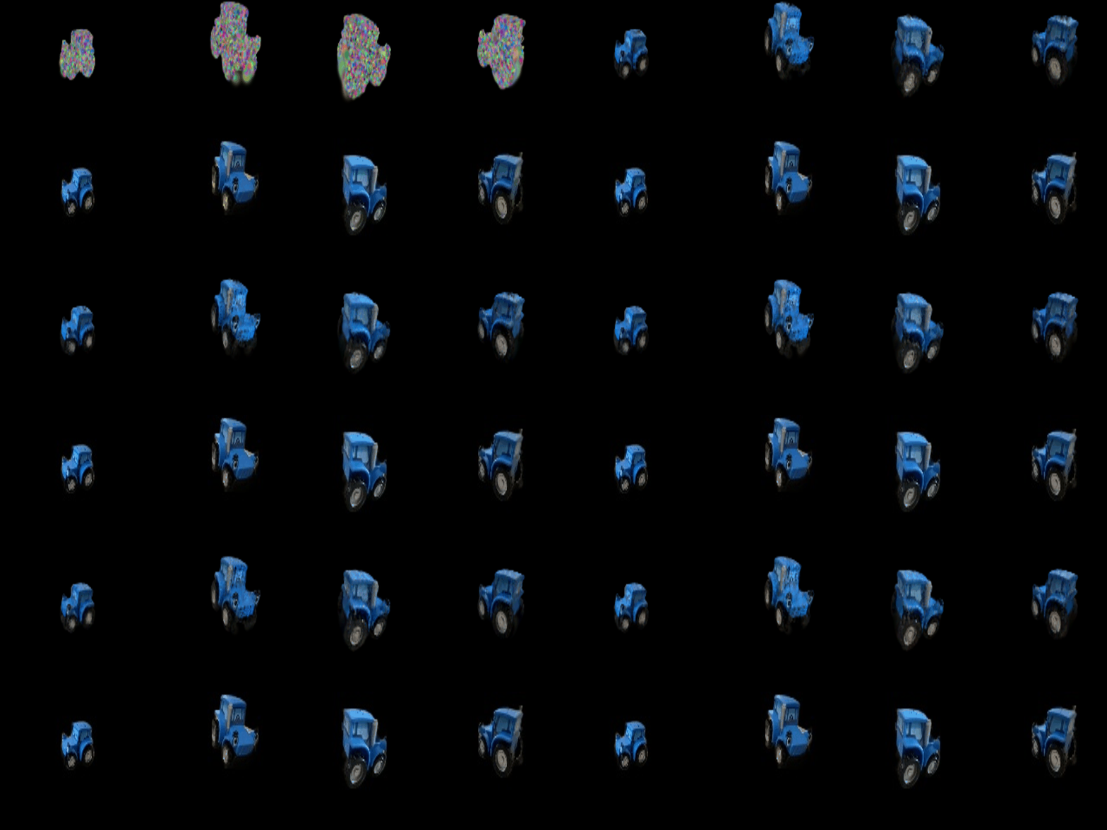

The full-batch rasterizer evaluates every Gaussian at every pixel and keeps all intermediates for
the backward pass; the README estimates about 15.5 GB for this, more than the 10 GB of
the RTX 3080 used here. Each mini-batch splat
is therefore wrapped in torch.utils.checkpoint (1000 Gaussians per splat), which
recomputes its intermediates during backward instead of storing them. The result is unchanged;
training is slower.
Colours are evaluated from all 16 SH coefficients per channel (degree 3), using the normalized direction from the camera centre to each Gaussian, then offset by 0.5 and clamped at 0.

Each comparison below shows the DC-only render on the left and the full-SH render on the right, from the same camera.


Materials scene at 128×128, 10k Gaussians with init_type="random", evaluated on
the 100 validation views. The baseline is the Q6 setup unchanged (isotropic, L1, the Q6 learning
rates, 1000 iterations; train_harder_scene.py --baseline).
| Materials | Iterations | PSNR | SSIM |
|---|---|---|---|
| Baseline (Q6 setup) | 1000 | 18.23 | 0.685 |
| Improved | 3000 | 23.75 | 0.876 |
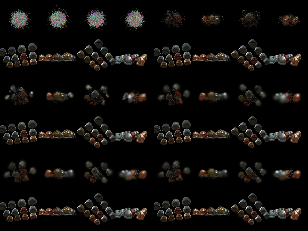
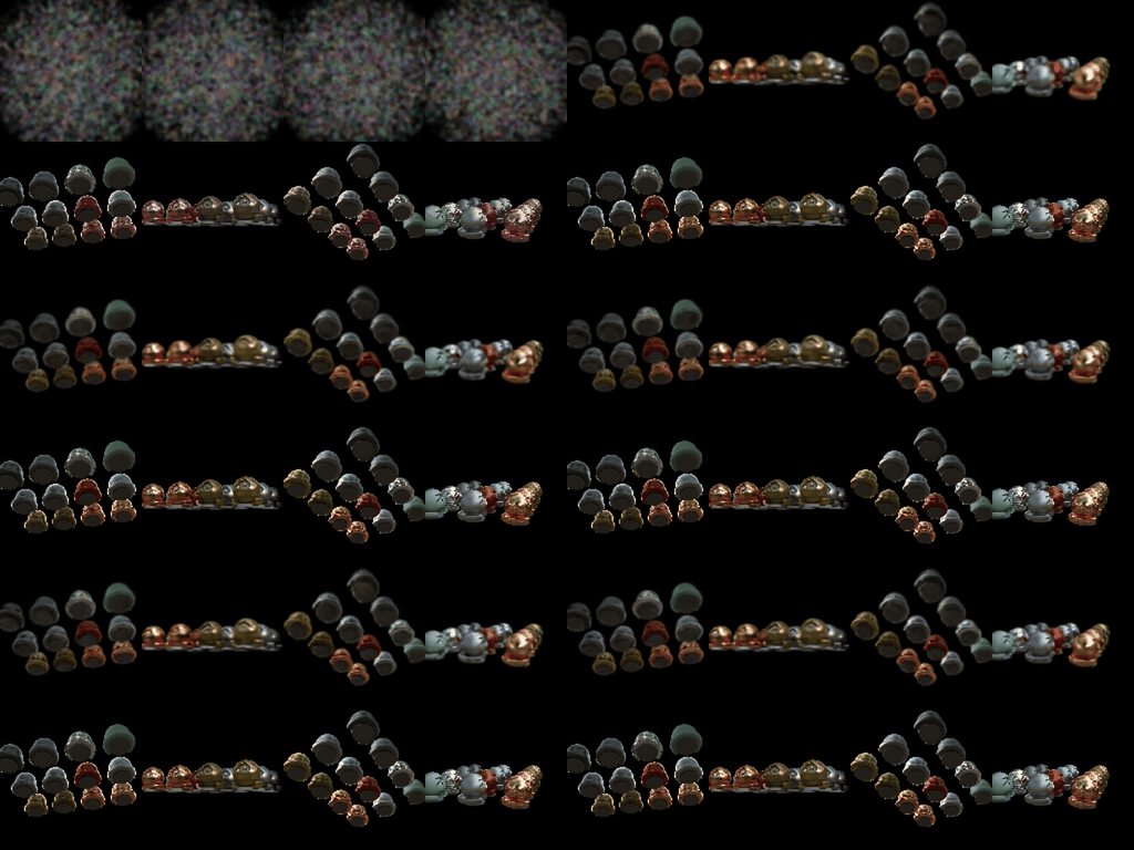


The default random init draws means from N(0, 0.2²), nearly opaque (sigmoid(8))
and tiny. The spheres span roughly ±1.5 units, so almost every Gaussian starts inside the
centre of the scene. The baseline ends with blurry blobs clustered around the middle spheres,
which suggests that at the Q6 learning rate the means do not move far enough from this start. Modifications, in
the improved run:
These were applied together and not ablated one at a time (each run takes 30–85 minutes on this GPU), so the gain is not attributed to individual changes. Adaptive density control (cloning, splitting and pruning) was not used.