Assignment 3 - Fall 2026
Karthik Srinivasan (ksriniv2)
Compute: NeRF part on my laptop (RTX 3060 Laptop GPU, 6 GB). The Gaussian splatting render and training runs were done on an RTX 5090.
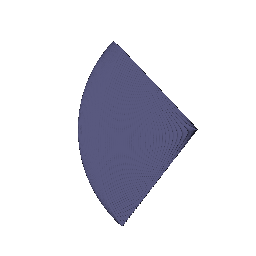
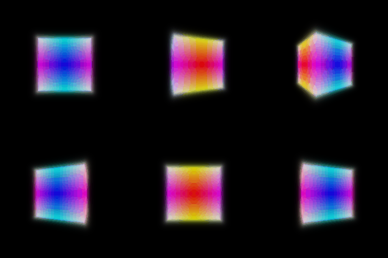
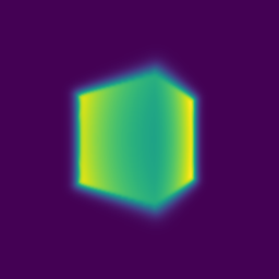
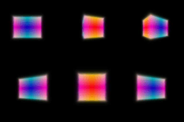
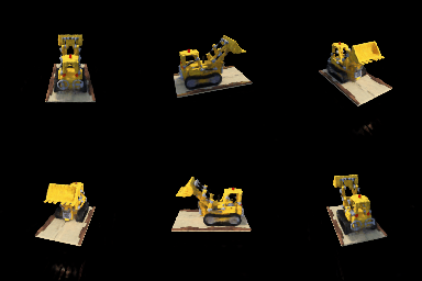
Density depends only on position. The colour head gets the position feature plus the harmonic embedded, normalized ray direction.
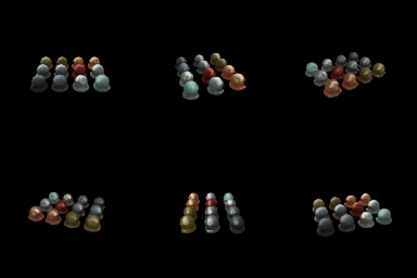
The shiny parts of the spheres change with the camera angle, which a colour that only depends on position cannot do.
More view dependence lets the model fit highlights, but it can hurt generalization. With only a few training views, a network that sees the direction can fit each training view's colours separately and look wrong from new angles. Following the standard NeRF design, the direction only goes into the last small colour head and density depends on position alone, so the geometry stays consistent across views and only the colour can vary with direction.
Setup: 64 coarse samples per ray, then 64 fine samples drawn from the coarse weights and merged with the coarse ones, so the fine network sees 128 points per ray. The loss is the fine MSE plus the coarse MSE.
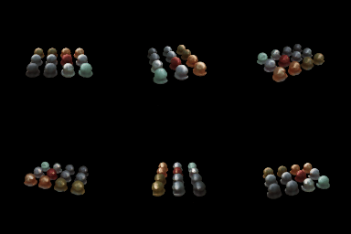
The fine samples land near the surface, so they are used where they matter. The cost is a second network and a second pass. Per ray, the coarse network runs on 64 points and the fine network on the 128 merged points, so 192 network evaluations in total, compared to 128 for a single network with 128 uniform samples. Each training step costs more. In return the fine samples are placed where the density is, so more of the budget goes to the surface instead of empty space.
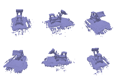
Geometry:
Color:
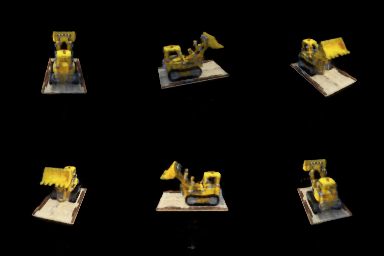
Settings: alpha = 10.0, beta = 0.05, eikonal weight = 0.02, 250 epochs, the defaults in volsdf_surface.yaml. I only ran these because I did not have time to try others, like different beta values and eikonal weights.
What alpha and beta do. Alpha is the density inside the object, so it sets how opaque it is. Beta sets how sharp the surface is: small beta makes density jump from 0 to alpha at the surface, large beta spreads it into a soft band.
1. How does high beta bias your learned SDF? What about low beta? With high beta the density is smooth and spread out, so the learned SDF is biased toward a blurry, smoothed surface that loses fine detail and can sit slightly off the true surface. With low beta the density is almost a step at the zero level set, so the SDF follows the surface closely, but it can become noisy and sharp.
2. Would an SDF be easier to train with volume rendering and low beta or high beta? Why? High beta is easier. Density is nonzero over a wide band, so many sample points along a ray get a useful gradient and the optimization is smooth. With low beta, only samples very close to the surface have any density, so most samples give almost no gradient and training is harder and less stable.
3. Would you be more likely to learn an accurate surface with high beta or low beta? Why? Low beta. The density is concentrated at the zero level set, so the rendered surface matches the SDF zero level set closely and gives a sharper and more accurate surface. High beta blurs the surface, so the SDF zero level set is less precisely pinned down.
| Parameter | Learning rate |
|---|---|
| Opacities | 0.05 |
| Scales | 0.01 |
| Colours | 0.02 |
| Means | 0.001 |
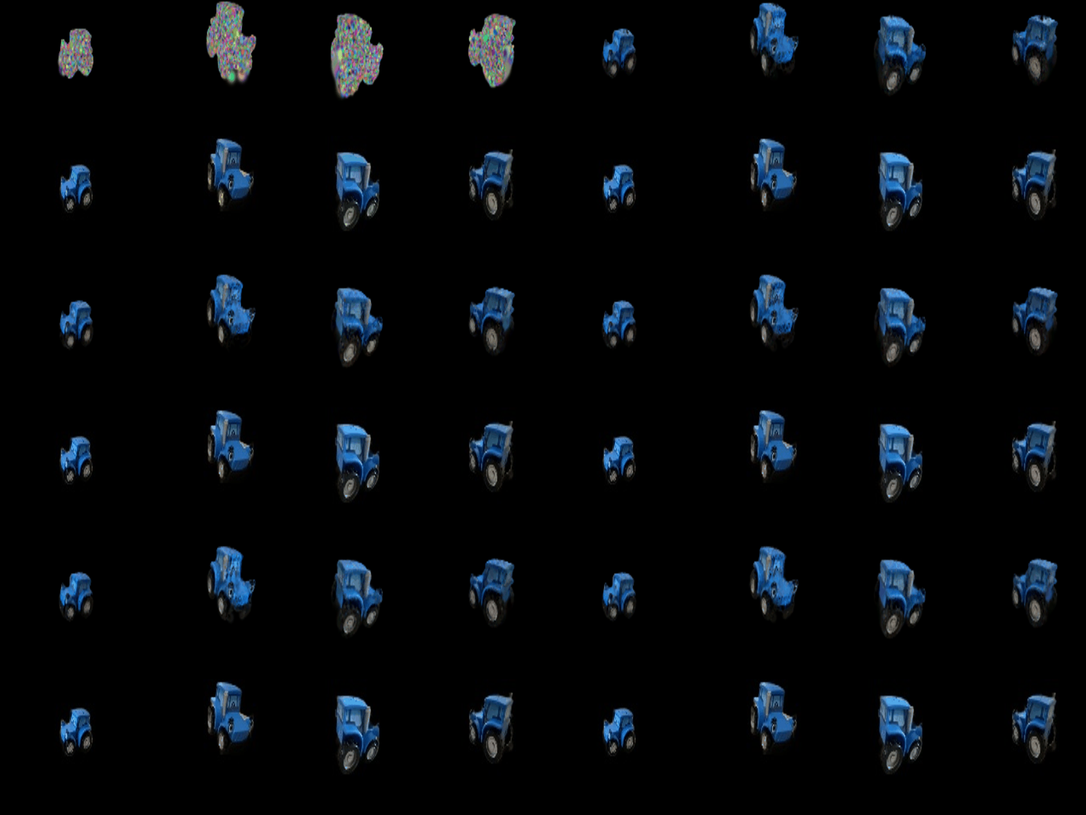
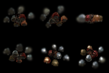
Training progress:
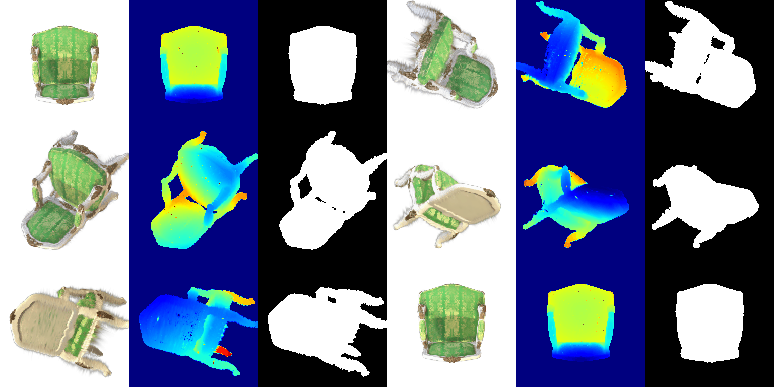
Final renders:

render.py GIF with spherical harmonics (7.1):
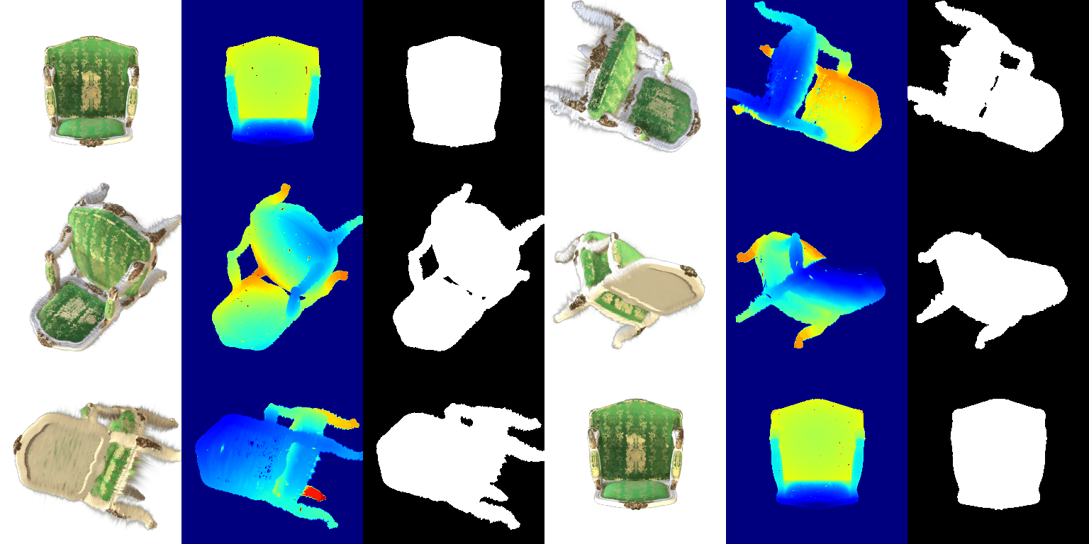
render.py GIF without spherical harmonics (5.5):
Side by side comparisons (left: without SH, right: with SH):
Frame 0
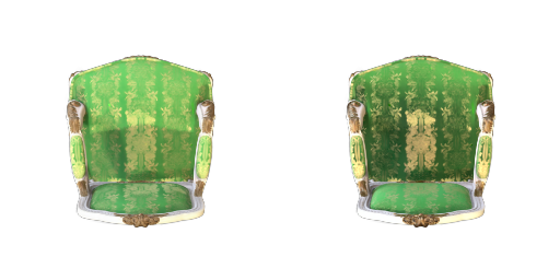
With SH the green cloth has more contrast: darker green in the shadowed areas and a brighter, sharper gold pattern. Without SH the back of the chair looks flatter and lighter.
Frame 8
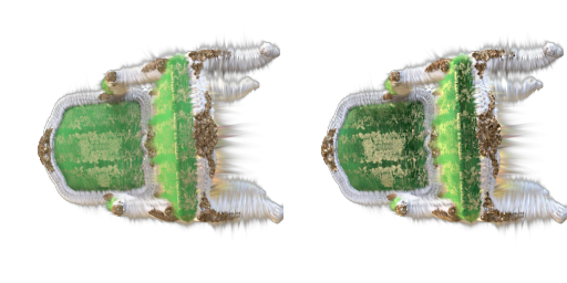
The two are very close. With SH the green on the seat is a little darker and has slightly more variation.
Frame 20
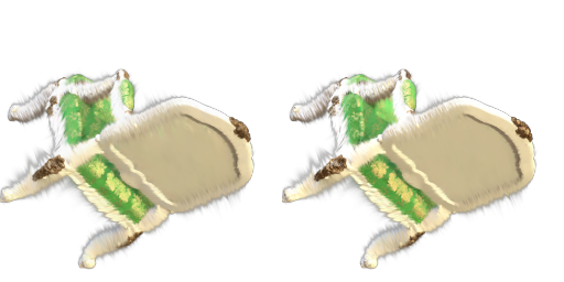
Again very close. The only difference I see is a small change in the shade of the green pattern, which is a bit deeper with SH.
Without SH each Gaussian has one fixed colour. With SH the colour depends on the viewing direction, so the differences show up as shading changes on the cloth, mostly where the view is close to the front.
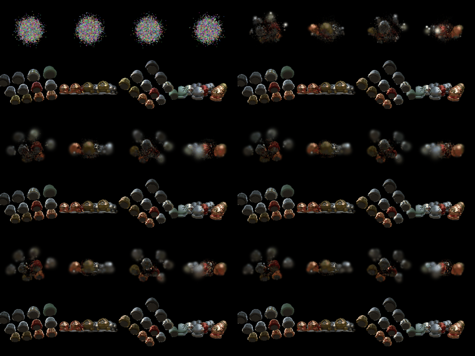
Random initialization of 10000 isotropic Gaussians on the materials scene. Baseline uses the Q6 settings. The only change I made is the learning rate of the means, from 0.001 to 0.02.
| Means LR | PSNR | SSIM | |
|---|---|---|---|
| Baseline | 0.001 | 18.347 | 0.696 |
| Improved | 0.02 | 20.568 | 0.723 |
Baseline:
Improved:
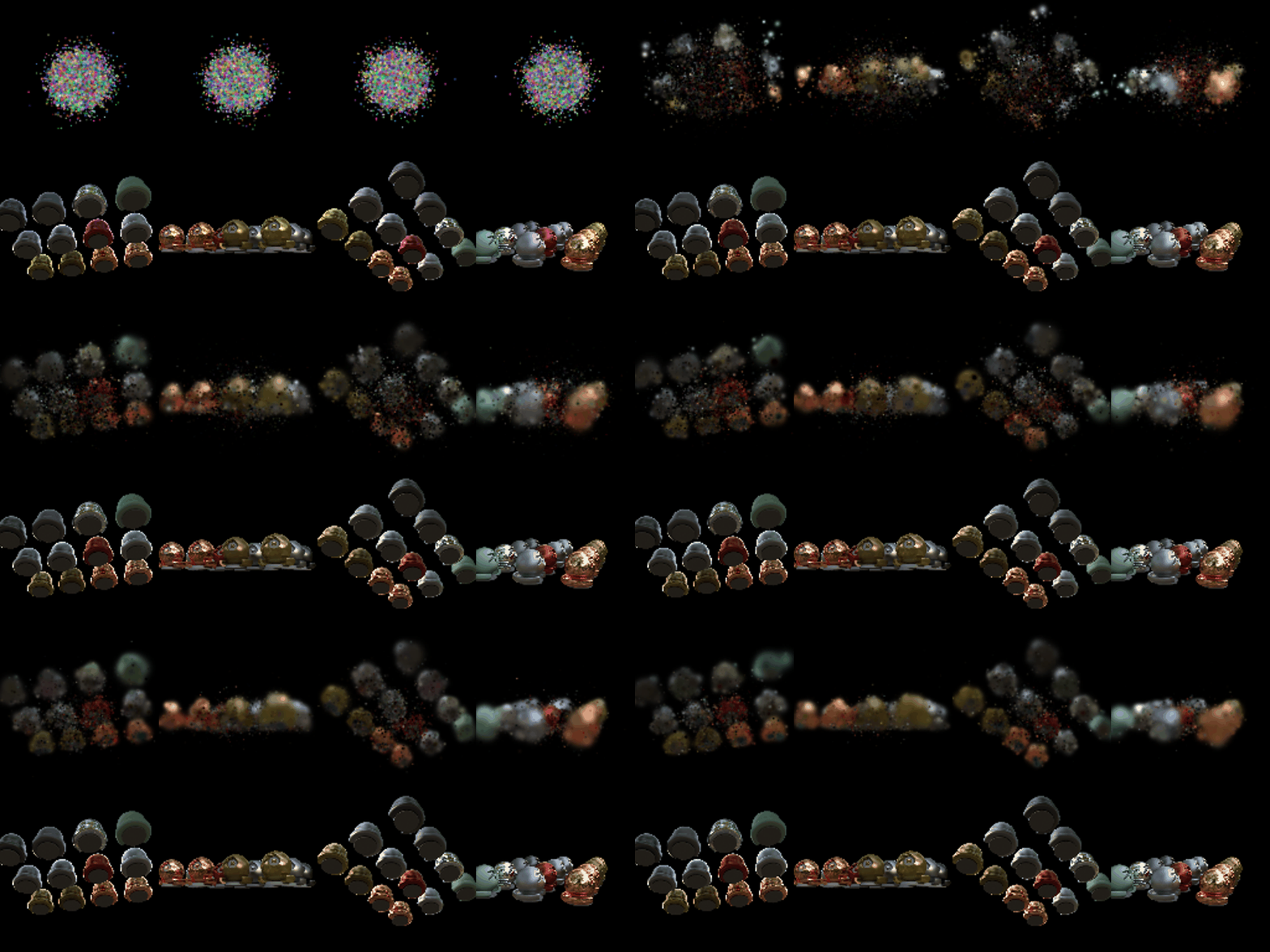
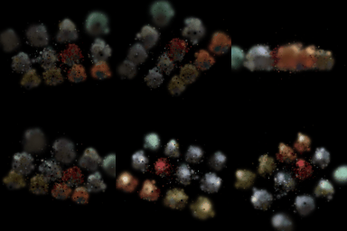
I did not have much time, so I only tried this one change. The Gaussians start at random positions, so the means need to move a lot, and the small learning rate was too slow in 1000 iterations. With more time I would have run means learning rates of 0.01 and 0.05, and a longer run of 3000 iterations.