Learning
to render.
From continuous neural fields to explicit Gaussian primitives. A study of differentiable rendering, appearance, and geometry.


Differentiable volume rendering
From camera pixels to an emission–absorption image.
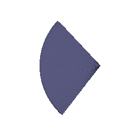
I generated normalized pixel coordinates, unprojected them into world space, and normalized directions from the camera center. Uniform distances produce sample points along each ray.
Transmittance uses an exclusive accumulated optical depth, so the first sample has T = 1. Weighted sums produce RGB and depth; depth is divided by its maximum for display.




Recovering a basic volume
Learning box geometry from posed RGB images.
I randomly selected pixels without replacement and minimized RGB mean squared error to optimize the box center and side lengths. Training ran for 1,000 epochs; the last displayed loss was approximately 10⁻⁶.
| Parameter | x | y | z |
|---|---|---|---|
| Center | 0.25 | 0.25 | 0.00 |
| Side lengths | 2.01 | 1.50 | 1.50 |


Neural radiance field
Replacing an analytic box with a learned scene function.
A position-only MLP maps harmonic encodings of 3D samples to density and RGB. Six harmonic frequencies give 39 input features. The six-layer position network uses 128 hidden units and a skip connection at layer index 3. ReLU ensures nonnegative density; Sigmoid bounds RGB.

Beyond a basic NeRF
View-dependent appearance, hierarchical sampling, and signed-distance geometry.
4.1 · View dependence
I concatenate a low-frequency direction encoding with position features only in the shallow color head. Density remains independent of viewing direction. This allows highlights and reflections to change with the camera without making geometry direction-dependent.
Additional directional capacity can fit reflective appearance, but can also memorize training views. A small direction encoding and shallow head limit this flexibility. The materials sequence below demonstrates view-dependent rendering; without a matched held-out ablation, it does not establish a quantitative generalization gain.

4.2 · Coarse / fine sampling
Two independent networks are supervised by the sum of their RGB MSE losses. The coarse network evaluates 64 samples. Its detached interior weights define a PDF for 64 additional samples; the fine network evaluates the sorted union of 128 points. Training jitters coarse distances; evaluation uses deterministic samples.
Importance sampling concentrates evaluations near contributing surfaces. The trade-off is a second network and 192 total network sample evaluations per ray, compared with 128 for the original single network. It can improve sample placement, but speed and quality gains require measurement rather than being guaranteed.

4.3 · VolSDF
Separate encoded MLPs predict signed distance and color. Signed distance has no final activation; color uses Sigmoid. I convert distance to density using a scaled Laplace CDF and add an Eikonal penalty E[(‖∇f‖ − 1)²].
| Setting | Value |
|---|---|
| Training | 250 epochs · Adam · 0.0005 |
| Density parameters | α = 10 · β = 0.05 |
| Eikonal weight | 0.1 |
| Initialization | 1,000 steps fitting a unit-sphere SDF |
| Distance / color MLP | 6 layers × 128 / 2 layers × 128 |
| Eikonal sampling bounds | [−4, 4]³ |


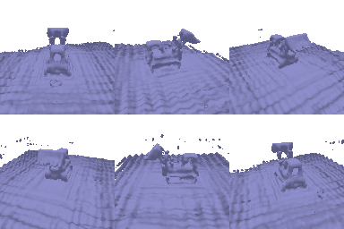
The first random initialization produced extensive unwanted surfaces. Sphere pretraining and stronger Eikonal regularization reduced these artifacts. The final mesh remains simplified and the RGB result is softer than the density NeRF, so the surface reconstruction is not fully resolved.
Initial VolSDF failure

Understanding α and β
α controls density magnitude. Larger α makes the interior more opaque. β controls transition width. High β spreads density across a wider band and can bias image formation toward diffuse, less localized surfaces. Low β approximates a sharper inside/outside transition.
Training: a moderately high β generally offers a wider region of useful gradients and is easier to optimize with finite samples. Very low β needs samples close to the surface and can make optimization unstable. Accuracy: a lower β can localize a surface more precisely after convergence, but only if sampling and optimization resolve that narrow transition; low β alone does not guarantee better geometry.
3D Gaussian rasterization
Project, sort, evaluate, and composite.
I construct 3D covariance matrices from scales and rotations, project means into screen coordinates, and propagate covariance through the camera transform and projection Jacobian. A 0.3 diagonal floor limits subpixel footprints. Isotropic covariance reduces to s²I.
Camera-space depth filters Gaussians behind the camera and orders the remainder front to back. At each pixel, opacity multiplies the exponential quadratic form; exclusive transmittance gives compositing weights. The same weights aggregate RGB, depth, and silhouette. Mini-batches carry transmittance including the final Gaussian; residual transmittance blends the background once.

Training Gaussian representations
Fitting a toy truck from a point-cloud initialization.
I initialize 10,000 isotropic Gaussians from the supplied point cloud and optimize positions, log scales, opacity logits, and RGB using L1 image loss. Rotations remain fixed because isotropic Gaussians are rotation invariant.
| Iterations | Held-out PSNR | Held-out SSIM |
|---|---|---|
| 1,000 | 28.444 dB | 0.929 |
| Parameter | Learning rate |
|---|---|
| Means | 0.0001 |
| Log scales | 0.005 |
| Opacity logits | 0.01 |
| Colors | 0.01 |


Appearance with spherical harmonics
The same geometry, viewed with a richer color model.
I load all 16 real SH coefficients per color channel through degree 3 and evaluate them along normalized camera-to-Gaussian directions. The weighted basis sum plus 0.5 produces RGB, clamped below at zero. Coefficients are pretrained; this experiment performs inference only.

Matched-view RGB comparisons


The SH rendering subtly changes the green upholstery shading and edge contrast; the DC version has a more uniform appearance.


The oblique view shows small direction-dependent tonal changes along the seat and frame. Silhouette and geometry remain the same.


From this view, differences are mainly in local shading rather than object shape. SH preserves the geometry while adjusting RGB with direction.
A harder scene: materials
Random initialization, multiple objects, and anisotropic refinement.
The baseline transfers the truck settings to 10,000 randomly initialized isotropic Gaussians. The improved experiment keeps 10,000 Gaussians and L1 loss, but uses anisotropic scales and trainable rotations, broader random scene coverage, lower initial opacity, and exponential learning-rate decay.
| Method | Iterations | Validation PSNR ↑ | Validation SSIM ↑ |
|---|---|---|---|
| Isotropic baseline | 1,000 | 19.524 dB | 0.669 |
| Anisotropic experiment | 1,000 | 21.696 dB | 0.786 |
| Change | Same budget | +2.172 dB | +0.117 |
Higher validation PSNR after changing initialization and optimization together.
Training progress


| Setting | Baseline | Improved |
|---|---|---|
| Random positions | Gaussian cloud near origin, std 0.2 | Uniform ball, radius 1.5 |
| Initial scale | Random, approximately 0–0.01 | 0.03 per axis |
| Initial opacity | sigmoid(8) ≈ 1 | 0.1 |
| Shape | Isotropic | Anisotropic; trainable rotations |
| Means LR | 0.0001 | 0.001 → 0.0001 |
| Scales LR | 0.005 | 0.003 → 0.0003 |
| Opacity / color LR | 0.01 | 0.01 → 0.001 |
| Rotation LR | Fixed | 0.001 → 0.0001 |
| Loss | L1 | L1 |
| Scale bounds | No extra bounds | 0.003–0.3 |
| Color bounds | No extra bounds | Clamped to [0, 1] |
Broader initialization places Gaussians near more objects, while larger initial footprints provide gradients over a wider image region. Lower initial opacity reduces early occlusion. Anisotropy provides more flexible surface coverage, and learning-rate decay allows larger early updates followed by refinement.
The combined method improves both reported validation metrics at the same iteration budget. Because several settings changed together and the baseline was not explicitly seeded in the starter loop, this is a combined-method comparison rather than a controlled attribution of the gain to anisotropy alone. Remaining errors include fine detail and view-dependent reflections; the training model uses RGB colors rather than learned SH.