
Name: Kashish Gandhi
Andrew ID: kgandhi2
This assignment studies several ways to represent and reconstruct a 3D object from one RGB image. I first optimized voxel, point-cloud, and mesh representations directly using representation-specific losses. I then trained image-conditioned decoders for all three representations, analyzed a mesh smoothness hyperparameter, visualized learned behavior, and implemented implicit and parametric decoders.
I used the provided pretrained ResNet-18 image features with
--load_feat. Training was performed primarily with Apple
MPS, while evaluation and visualization were run on CPU for
compatibility.
For voxel fitting, I used binary cross-entropy with logits. Each grid entry is treated as a binary occupancy label:
\[ \mathcal{L}_{\text{voxel}} = -\frac{1}{N}\sum_i \left[y_i\log \sigma(\hat y_i) + (1-y_i)\log(1-\sigma(\hat y_i))\right]. \]
The optimized grid captures the coarse occupied volume of the target. Its main limitation is the fixed \(32^3\) spatial resolution, which makes thin chair structures appear blocky.
I implemented the symmetric Chamfer distance. For predicted points \(P\) and target points \(Q\):
\[ \mathcal{L}_{\text{Chamfer}}(P,Q) = \frac{1}{|P|}\sum_{p\in P}\min_{q\in Q}\|p-q\|_2^2 + \frac{1}{|Q|}\sum_{q\in Q}\min_{p\in P}\|q-p\|_2^2. \]
The two directional terms are both necessary: one keeps predicted points near the target, while the other encourages coverage of the complete target surface.

The mesh objective combines Chamfer distance between sampled surface points with mesh Laplacian smoothing:
\[ \mathcal{L}_{\text{mesh}} = \lambda_c\mathcal{L}_{\text{Chamfer}} + \lambda_s\mathcal{L}_{\text{smooth}}. \]
Chamfer loss moves the surface toward the target, while smoothing discourages neighboring vertices from forming irregular spikes. The fitted mesh remains topologically constrained by its initial template.

All models use the same pretrained image feature vector but decode it into different 3D representations. Evaluation samples points from the prediction and ground-truth mesh and computes precision, recall, and F1 over multiple distance thresholds.
The voxel decoder uses a fully connected layer followed by 3D transposed-convolution blocks that progressively upsample the image feature into a \(32\times32\times32\) occupancy grid. The model captures the overall occupied volume but loses narrow structures because of voxel discretization.
Final F1@0.05: 56.971


The point decoder maps the 512-dimensional image feature through an
MLP and directly predicts n_points × 3 coordinates. Chamfer
distance provides a permutation-invariant training objective. Point
clouds represent surface detail more flexibly than voxels, although they
do not explicitly encode connectivity.
Final F1@0.05: 77.100


The mesh model begins with an icosphere template and predicts an XYZ displacement for every template vertex. The output preserves a connected surface, and the loss combines sampled-surface Chamfer distance with Laplacian smoothing.
Final F1@0.05: 70.660


| Representation | F1@0.05 | Main advantage | Main limitation |
|---|---|---|---|
| Voxel | 38.792 | Stable volumetric occupancy | Resolution limits thin details |
| Point cloud | 77.100 | Flexible surface coverage | No explicit connectivity |
| Mesh | 70.660 | Connected, renderable surface | Fixed topology and harder optimization |
The point-cloud model achieved the highest F1 (77.100) because Chamfer loss directly optimizes distances between predicted and ground-truth surface samples. The mesh model ranked second (70.660): its connected-surface prior is useful, but deforming a fixed sphere into chairs with different topology is difficult. The voxel model obtained the lowest score (38.792) because geometry is quantized into a fixed grid, causing narrow legs and armrests to disappear or become overly thick. Smoothness introduces an additional mesh tradeoff: it removes unstable spikes but can suppress valid thin geometry.
I varied the Laplacian smoothness weight while keeping the architecture, data, and Chamfer weight fixed.
| Smoothness weight | F1@0.05 | Qualitative behavior |
|---|---|---|
| 0.0 | 72.034 | Highest quantitative accuracy, but weakest regularization |
| 0.1 | 69.925 | Moderate smoothing with a small reduction in F1 |
| 1.0 | 65.589 | Strongest smoothing and lowest F1 |


The no-smoothing model achieved the highest F1@0.05, and F1 decreased as the smoothness weight increased. This indicates that the sampled-surface metric rewards close geometric fitting more than triangle regularity. Smoothness is still a useful visual prior: it can suppress spikes and irregular local deformations, but excessive smoothing removes thin chair structures and moves surface samples away from the ground truth. Thus, \(w_{smooth}=0.0\) was best quantitatively in this experiment, while a small nonzero weight may still produce cleaner meshes qualitatively.
To inspect more than final predictions, I visualized how the mesh changes as smoothness strength varies. This reveals which geometric structures are learned confidently and which are mainly controlled by the regularizer. Broad regions such as seats and backs remain relatively stable, while thin legs, armrests, and local high-curvature regions change substantially. These sensitive regions are also where a single RGB view provides the greatest depth ambiguity.
I also created a per-point error heatmap. It colors the predicted point cloud by nearest-neighbor distance to the ground truth, making it easy to locate failure regions rather than reducing the entire reconstruction to one score. High-error regions tend to occur on thin legs, armrests, and occluded surfaces.


The feature-interpolation visualization linearly interpolates between two image feature vectors and decodes intermediate point clouds. A smooth geometric transition indicates that the decoder has learned a structured latent space rather than memorizing isolated training examples.

 Together, these
visualizations suggest that the network learns a strong category-level
chair prior, but is less certain about occluded and thin geometry. It
produces plausible chairs even when every invisible detail cannot be
recovered from one image.
The implicit decoder represents shape as a function rather than directly predicting a structured voxel tensor:
\[ f_\theta(\mathbf{x},\mathbf{z}) \rightarrow o, \]
where \(\mathbf{x}=(x,y,z)\) is a location in normalized 3D space, \(\mathbf{z}\) is the image feature, and \(o\) is an occupancy logit. I created a \(32^3\) query grid over \([-1,1]^3\), concatenated every coordinate with the image feature, and evaluated the MLP at all 32,768 locations.
Because occupied voxels are much less common than empty voxels, an unweighted binary cross-entropy objective can collapse to predicting empty space everywhere. I therefore used a positive-class-weighted occupancy loss for the implicit model while leaving the original voxel loss unchanged.
Final F1@0.05: 15.687


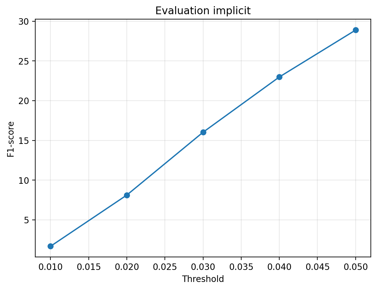
The implicit formulation provides a coordinate-conditioned representation and is conceptually resolution-independent. In this implementation, however, the function is evaluated only on a \(32^3\) grid for comparison with the voxel baseline. Its F1@0.05 of 15.687 was substantially lower than the explicit point and mesh models. The result highlights the sensitivity of occupancy networks to class imbalance, coordinate conventions, surface-extraction threshold, and training duration. The model often learned coarse occupancy but struggled to recover thin chair geometry accurately.
The parametric decoder maps a sampled 2D domain into 3D:
\[ g_\theta(u,v,\mathbf{z}) \rightarrow (x,y,z). \]
I sampled a regular 2D grid, concatenated each \((u,v)\) location with the image feature, and used an MLP to predict its corresponding 3D point. The output was trained with symmetric Chamfer loss against points sampled from the ground-truth mesh.
Final F1@0.05: 70.577


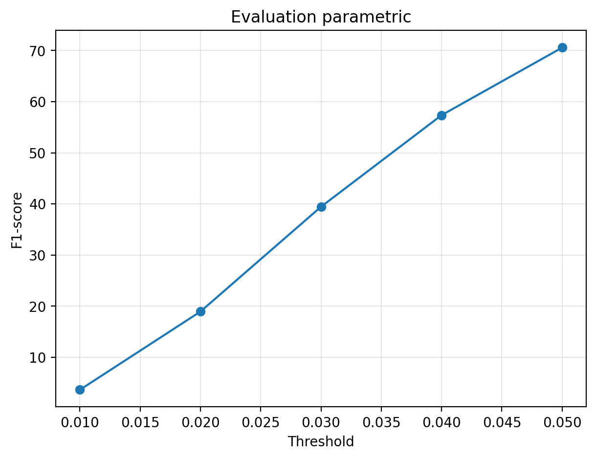
Unlike the standard point decoder, each predicted point is associated with a position in a shared 2D parameter domain. Nearby parameter samples can learn related 3D locations, introducing an implicit organization of the output. The parametric model achieved an F1@0.05 of 70.577, lower than the direct point-cloud decoder’s 77.100 but close to the mesh model’s 70.660. This suggests that the 2D domain provides useful structure, although a single patch has difficulty representing chair surfaces that require multiple charts. The current output also does not explicitly construct mesh faces.
I trained the point-cloud reconstruction model on the extended dataset containing chairs, cars, and airplanes. To make the comparison with the original chair-only model controlled and meaningful, I evaluated the three-class-trained checkpoint on the same 678 chair test examples used by the single-class experiment.
| Training data | Representation | Chair test examples | F1@0.05 |
|---|---|---|---|
| Chair only | Point cloud | 678 | 77.100 |
| Chair + car + airplane | Point cloud | 678 | 76.197 |


The chair F1 score decreased by only 0.903 points, from 77.100 to 76.197, after extending training to three object categories. This small reduction is expected because a fixed-capacity decoder must represent substantially more shape diversity instead of specializing only in chairs. At the same time, multi-class training makes the model more broadly useful and encourages a latent representation shared across categories. The close chair scores show that this additional diversity was learned without a major loss of chair reconstruction quality. These reported numbers are specifically a controlled chair-test comparison; a category-balanced test over all three classes would additionally be needed to report overall multi-class performance.
The experiments show that representation choice strongly affects both optimization and output geometry. Voxels are simple and stable but resolution-limited; point clouds optimize surface coverage directly but lack topology; and meshes provide connected surfaces but impose a difficult template-deformation problem. The implicit model offers a flexible function-based view of occupancy but requires careful handling of class imbalance. The parametric model adds structure to point prediction through a 2D domain, although a richer multi-patch design would better represent complex chair surfaces.
--load_feat.