16-825: Assignment 2
Kaushik Chavali (kchavali)
1. Exploring Loss Functions
1.1 Fitting a voxel grid
Binary cross entropy with logits was used for voxel occupancy.


1.2 Fitting a point cloud
Symmetric Chamfer distance was used for point-cloud fitting.


1.3 Fitting a mesh
Chamfer distance with Laplacian smoothing was used for mesh fitting.


2. Reconstructing 3D from a Single View
All baseline models use a pretrained ResNet-18 image encoder with separate voxel, point-cloud, and mesh decoders. The following sections show three test examples and the F1 results for each representation.
Default training hyperparameters
Unless otherwise stated, models were trained for 10,001 iterations with Adam, a learning rate of $4\times10^{-4}$, batch size 32, 1,000 sampled points, and checkpoints saved every 2,000 iterations. The implicit model used batch size 8 because it evaluates all $32^3$ query coordinates for every image. Mesh training used Chamfer weight 1.0 and smoothness weight 0.1. The four-patch parametric model used 250 points per patch.
2.1 Image to voxel grid
The decoder uses four 3D transposed convolutions to produce a $32^3$ occupancy grid.

Test examples
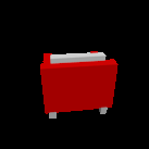


The voxel model captures coarse occupancy but often loses thin chair legs and gaps.
2.2 Image to point cloud
An MLP maps each image feature to 1,000 XYZ coordinates.

Test examples
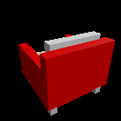


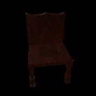


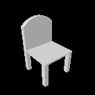


The point model obtains the strongest baseline result and preserves thin structures better than the voxel model.
2.3 Image to mesh
The mesh decoder predicts vertex offsets for a level-4 icosphere.

Test examples
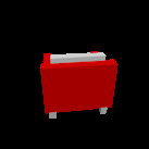


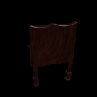


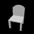


Baseline comparison
Point clouds perform best (~79.8), followed by meshes (~72.8) and voxels (~57.5). Point prediction avoids voxel quantization and fixed mesh topology. Meshes provide connected surfaces, while the $32^3$ voxel resolution loses the most thin geometry.
2.4 Effect of initial mesh resolution
I varied the icosphere subdivision level: level 3 has 642 vertices, the level-4 baseline has 2,562, and level 5 has 10,242.


Increasing resolution from level 3 to level 4 produces a clear improvement because the decoder has enough vertices for chair details. Level 5 gives only a small additional gain despite roughly quadrupling the level-4 vertex count. The higher computational and parameter cost therefore has diminishing returns.
2.5 Interpreting the learned model
Multi-view consistency
The same chair was reconstructed by the point model from ten camera views. Each heatmap cell is the symmetric Chamfer distance between two predicted point clouds.

The largest yellow distances generally compare a back-facing view with a front or interior-facing view. Each image hides different geometry: a rear view provides little evidence about the seat and front structure, while a front view hides much of the back. The model therefore completes these unseen regions differently. Most other pairs remain close, showing useful view consistency despite this single-view ambiguity.
Latent-space interpolation
I encoded two chair images, linearly interpolated their 512-D image features, and decoded every intermediate feature with the trained mesh decoder. No model was retrained during interpolation.


The chair changes continuously instead of jumping between two memorized outputs. The legs, seat, and back deform coherently from one chair to the other, supporting the conclusion that the encoder-decoder learned a structured global representation of chair shape. This does not prove that individual latent dimensions correspond to specific parts, and the fixed mesh topology also helps keep every intermediate surface connected.
3. Additional Architectures and Datasets
3.1 Implicit occupancy decoder
A fixed $32^3$ meshgrid supplies XYZ query coordinates in $[-1,1]^3$. The model projects the image feature, concatenates it with each coordinate, and uses a shared MLP to predict occupancy logits.


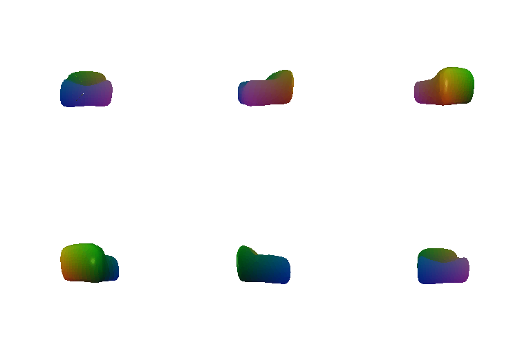





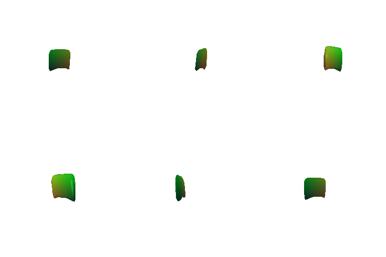

This simple coordinate MLP underperforms the convolutional voxel decoder. It lacks the strong local 3D spatial prior provided by transposed convolutions. Several outputs occupy only a small central region, and example 400 is empty at the 0.5 occupancy threshold.
3.2 Parametric patch decoder
Four independent MLPs each map 250 sampled UV points and the image feature to XYZ coordinates. Their outputs are concatenated into a 1,000-point cloud. Random UV samples are used during training and a fixed set during evaluation.


The parametric decoder is below the direct point decoder (~79.8) but remains competitive. Its UV parameterization encourages each MLP to learn a continuous surface patch, while independent patches allow different chair regions to specialize.
3.3 Extended three-class dataset
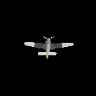
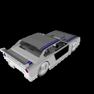
I trained the point decoder on chairs, cars, and airplanes, then evaluated it both on the full three-class test split and on the original chair-only test split.


Examples across classes




Same-chair qualitative comparison


Quantitative and qualitative analysis
On the same chair test split, the chair-only model reaches about 79.8 F1 and the three-class model reaches about 79.3, a decrease of only about 0.5 points. The one-class model is therefore slightly more specialized for chairs, but three-class training retains nearly all of its chair accuracy.
Qualitatively, both models recover the same major chair structure. In these examples the three-class predictions are sometimes slightly more diffuse, consistent with the small F1 decrease, but they do not collapse or lose chair identity. Across the complete dataset, the three-class model produces clearly different airplane, car, and chair geometry, so its output space is substantially more diverse while remaining category-consistent. The 87.6 aggregate full-split score is not directly comparable with chair-only F1 because the test classes differ.