Assignment 4 for 16-825 (Multi-View Transformers)
Experimental setup
- Data. The ScanNet++ iPhone subset from the course archive: 224 training, 28 validation and 28 test scenes. Every training sample has 8 views drawn in random order from a window of 32 consecutive frames, center-cropped to a square and resized to 224×224.
- Hardware. NVIDIA A100 80 GB GPUs, shared with other jobs on the same machine, so the wall-clock times below are slower than on a dedicated GPU. Everything runs on one GPU except the second stage of Mini-VGGT training, which uses two GPUs with DDP.
1. Multi-View Data Preprocessing (20 points)
Data visualizations
After unprojection. Points and cameras in the original ScanNet++ world frame, in meters (red frustum: first sampled camera). The 8 depth maps land on top of each other as one consistent point cloud.


After canonicalization. The same frames in camera 0's frame. The panel on the right of each screenshot shows the first camera centre at (0, 0, 0) and a valid-point centroid distance of 1.000.


Canonicalization, world-space ray directions and the Plücker moment
Canonicalization. Every pose is left-multiplied by the inverse of camera 0's pose, so camera 0 becomes the identity and all geometry is expressed in its frame. Translations, depth and points are then divided by the scene scale s, the distance from camera 0 to the centroid of the valid points, so that centroid ends up at distance 1. This removes the arbitrary origin, orientation and metric scale of each scan, which the images cannot tell the model anyway, so every sample follows the same convention and the models only have to learn relative geometry.
World-space ray directions. The camera-space direction of pixel (u, v) is K−1[u, v, 1]T. Rotating it by the camera-to-world rotation and normalizing gives d = normalize(R K−1[u, v, 1]T). Only the rotation applies, because a direction has no position: the camera centre t becomes the ray origin. Since the poses are canonical, all rays are in camera 0's frame.
Plücker moment. Each ray is stored as [d, m] with the moment m = o × d. The moment is the same whichever point of the line is used as the origin, since (o + λd) × d = o × d, so (d, m) describes the line itself. With a unit d, |m| is the line's distance from camera 0. The direction tells the model where a pixel looks and the moment where the camera is, which gives LVSM a dense per-pixel camera encoding.
Final check: check_data.py output
python scripts/check_data.py --config configs/scannetpp/iphone/data.json --split train --max-samples 4:
{
"split": "train",
"dataset_samples": 224,
"checked_samples": 4,
"samples": [
{
"sequence_name": "e050c15a8d_frame_007080",
"views": 8,
"resolution": 224,
"valid_depth_fraction": 0.9779127240180969,
"max_reprojection_error_px": 0.00010923630907200277,
"max_ray_reprojection_error_px": 0.00010235906665911898,
"centroid_distance": 1.0
},
{
"sequence_name": "5f99900f09_frame_002820",
"views": 8,
"resolution": 224,
"valid_depth_fraction": 0.9903116226196289,
"max_reprojection_error_px": 0.00012419754057191312,
"max_ray_reprojection_error_px": 9.650505671743304e-05,
"centroid_distance": 1.0
},
{
"sequence_name": "47b37eb6f9_frame_002720",
"views": 8,
"resolution": 224,
"valid_depth_fraction": 0.9609947800636292,
"max_reprojection_error_px": 0.0001224803418153897,
"max_ray_reprojection_error_px": 0.00011108566104667261,
"centroid_distance": 1.0
},
{
"sequence_name": "4c5c60fa76_frame_006690",
"views": 8,
"resolution": 224,
"valid_depth_fraction": 0.7516716122627258,
"max_reprojection_error_px": 9.5367431640625e-05,
"max_ray_reprojection_error_px": 9.045338083524257e-05,
"centroid_distance": 1.0
}
],
"batch_shapes": {
"rgb": [2, 8, 3, 224, 224],
"depth": [2, 8, 1, 224, 224],
"depth_valid": [2, 8, 1, 224, 224],
"K": [2, 8, 3, 3],
"frame_numbers": [2, 8],
"T_world_from_camera": [2, 8, 4, 4],
"original_world_from_reference": [2, 4, 4],
"scene_scale": [2],
"points_world": [2, 8, 3, 224, 224],
"ray_origins": [2, 8, 3, 224, 224],
"ray_directions": [2, 8, 3, 224, 224],
"plucker": [2, 8, 6, 224, 224]
}
}All point and ray reprojection errors are about 1e-4 px, well below the 0.01 px threshold, and every centroid distance is 1.0.
2. Novel-View Synthesis with Mini-LVSM (40 points)
Model and training settings (configs/lvsm.json, unchanged): patch size 8 (28×28 = 784 tokens per view), width 384, 8 blocks, head dimension 64, MLP ratio 4, QK-norm, 14.6M parameters. 2 source views and 6 target views per sample, batch size 4 (56 steps per epoch), 100 epochs. AdamW (learning rate 2e-4, weight decay 0.05, betas (0.9, 0.95)), 200 warmup steps, then cosine decay to 10% of the peak, gradient clipping at 1.0, bfloat16 autocast.
2.1 Overfitting (10 points)
Settings. One fixed training batch (4 clips, 2 source views and 6 targets each), trained for 2000 steps with the default model and optimizer settings, then evaluated on that same batch.
| Overfit batch | MSE | PSNR | SSIM |
|---|---|---|---|
| Average over the 2000 training steps | 0.00687 | 25.36 dB | – |
| After 2000 steps | 0.00088 | 30.84 dB | 0.869 |
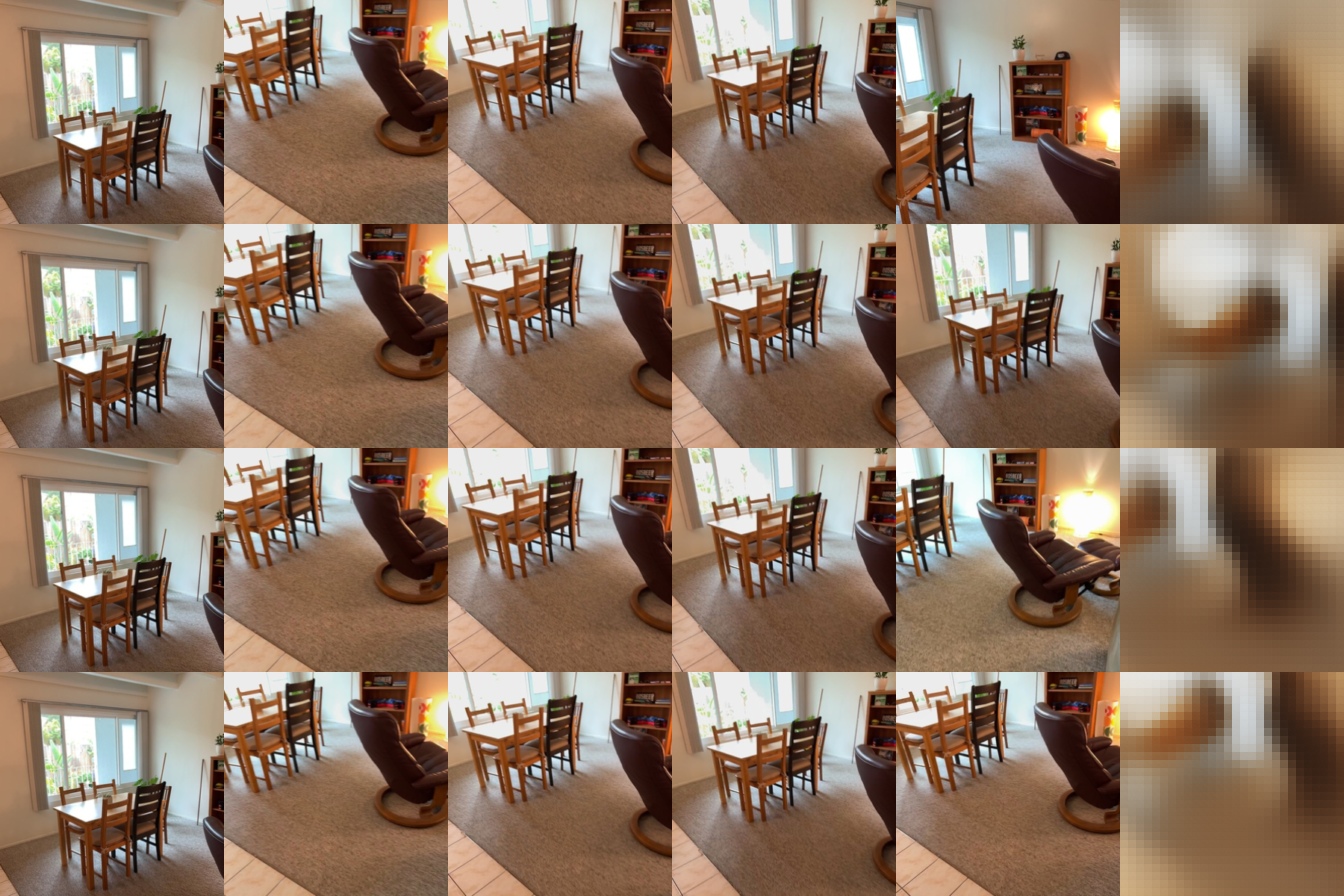
The final overfit PSNR is 30.84 dB, above the ~30 dB the check asks for. The training PSNR in the first row is lower because it is averaged over all 2000 steps, including the early ones where the model has not learned anything yet. The model can memorize a batch, so the tokens, rays and loss are wired correctly. In the visualization below (source views, ground truth, prediction), the predictions reproduce the batch closely: the chairs, the table, the lamp and the blue wall all line up with the ground truth. The remaining error is mostly faint 8×8 patch-grid artifacts and slightly soft edges, which are visible on the wall and the carpet.

val_epoch000.png after 2000 overfit steps: source views, ground truth, prediction 2.2 Training and evaluation (30 points)
Settings. The full training run uses the settings listed above: 2 source views and 6 targets per sample, 100 epochs on the training split (about 55 s per epoch, roughly 1.5 hours in total). Validation uses the fixed set of 28 validation clips, and best.pt is the checkpoint with the highest validation PSNR, which turned out to be the last epoch (99).

The loss drops quickly over the first 20 epochs, and after that it keeps improving slowly. Validation PSNR goes from 12.2 dB at epoch 0 to 16.15 dB at epoch 99, and SSIM from 0.38 to 0.56. Neither curve has flattened completely, so a longer schedule would probably still help. Validation PSNR stays slightly above training PSNR the whole time, so the model is not overfitting. The training number is averaged over randomly sampled clips while the weights are still changing during the epoch, whereas validation is measured at the end of the epoch on a fixed set of clips, so the two are not directly comparable.
Ablations. I evaluated best.pt on the validation split with 1, 2 and 4 source views, and with correct, shuffled and removed target rays. The model was only trained with 2 source views.
| Source views | Correct rays PSNR / SSIM | Shuffled rays PSNR / SSIM | No rays PSNR / SSIM | Target images |
|---|---|---|---|---|
| S = 1 | 15.20 / 0.558 | 11.80 / 0.487 | 12.47 / 0.527 | 196 |
| S = 2 | 16.15 / 0.560 | 11.49 / 0.472 | 12.44 / 0.527 | 168 |
| S = 4 | 16.89 / 0.576 | 11.60 / 0.474 | 12.44 / 0.537 | 112 |
Number of source views. With correct rays, quality goes up steadily with more source views: from 15.20 dB with one view to 16.15 dB with two and 16.89 dB with four. Even though the model was trained with only two source views, it uses the extra views at test time: the source tokens are just a longer sequence to attend over, and more views mean more of the target is actually visible in some source image. One caveat: with 8 views per clip, a larger S also means fewer and different targets (196, 168 and 112 images), so the three rows are not on exactly the same set of target images.
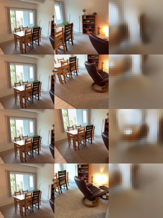
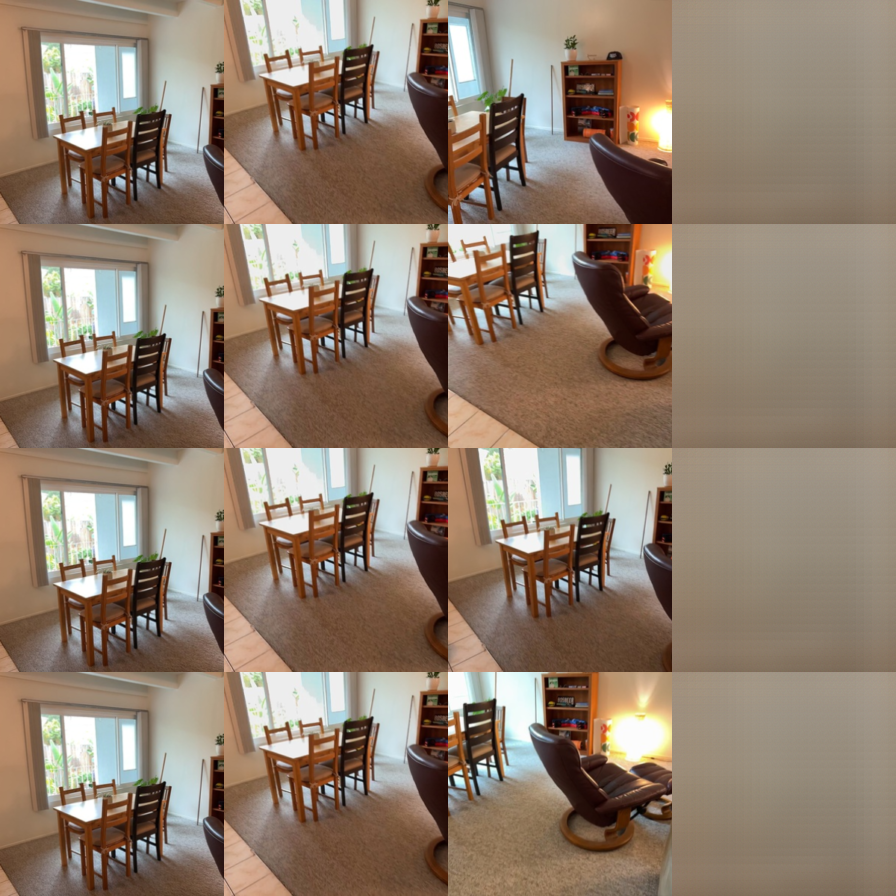
Ray conditioning. The target rays matter a lot. Removing them (all-zero rays) drops PSNR to about 12.4 dB for every S, and the number no longer changes with the number of source views. Without rays the model has no idea where the target camera is, so the best it can do is a blurry average of what the scene usually looks like, and the extra source views cannot help. Shuffling the rays is even worse (about 11.5–11.8 dB, the lowest SSIM): the model now confidently renders the view from a different target camera, which is further from the ground truth than a blurry average. In the shuffled visualization below, the predictions still look like this room, but the window, chair and floor sit in the wrong places for their own ground truth. Together these results show that the model really does use the Plücker rays to place the source content, and is not just copying or averaging the source images.
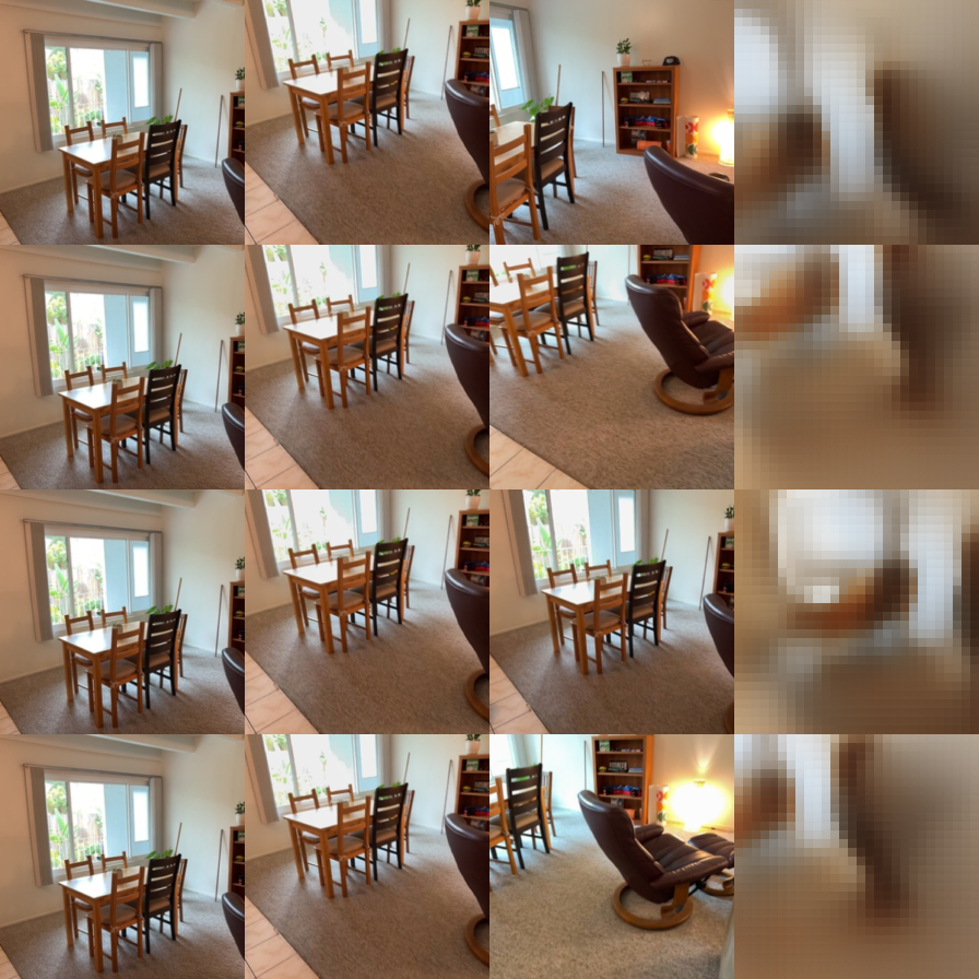
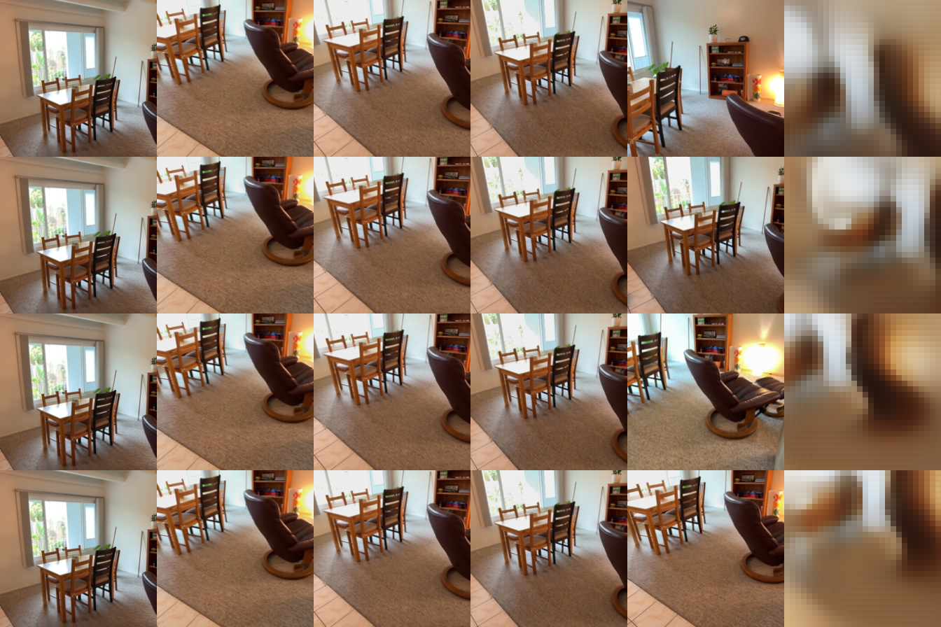
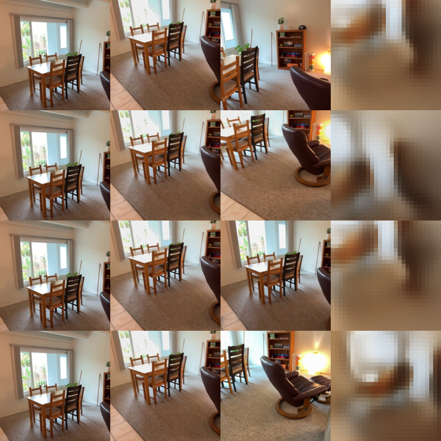
Visualizations. In every grid each row is one target view, and the columns are the source views, the ground truth and the prediction. The predictions get the overall layout and colours right (wall and window on the left, the dark chair, the carpet), but they are blurry and show visible 8×8 patch blocks, since a 14.6M-parameter model trained for 100 epochs cannot reproduce fine detail like chair legs or the bookshelf.


2.3 Bonus: training view count
Question. The ablation in 2.2 shows that a model trained with exactly 2 source views still improves when it gets 4 at test time. Does it help to train with a random number of source views, so the model sees every count it will be tested on?
Setup. Two runs that differ only in how the training clips are split into sources and targets:
- Fixed S = 2 (baseline): the default, 2 sources and 6 targets per clip.
- Random S: for every training step, S is drawn uniformly from {1, 2, 3, 4} and the remaining 8 − S views are targets. All clips in a batch share the same S. This is a small wrapper around the provided training script (
experiments/lvsm_random_views.py), which replaces only the source/target split of the training batches.
Everything else is identical: same model, same seed, same data order, 50 epochs each with the default optimizer and schedule (so the cosine decay completes within 50 epochs), and the two runs trained at the same time on two GPUs. Validation during training always uses S = 2, so the curves are directly comparable. At the end, best.pt of each run is evaluated with S = 1, 2, 3 and 4 and correct rays. 50 epochs is half of the 2.2 run, so absolute numbers are a bit lower than there (16.15 dB at S = 2 after 100 epochs).
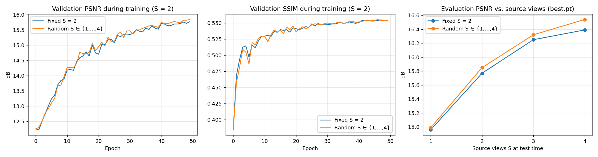
| Test-time S | Fixed S = 2 PSNR / SSIM | Random S ∈ {1,…,4} PSNR / SSIM | ΔPSNR | Target images |
|---|---|---|---|---|
| 1 | 14.96 / 0.553 | 14.99 / 0.553 | +0.03 | 196 |
| 2 | 15.77 / 0.554 | 15.85 / 0.553 | +0.08 | 168 |
| 3 | 16.25 / 0.557 | 16.32 / 0.556 | +0.07 | 140 |
| 4 | 16.39 / 0.568 | 16.54 / 0.566 | +0.15 | 112 |
Results. Training with a random view count is slightly better in PSNR for every test-time S, and the gap is largest with the most source views: +0.03 dB with one source view, +0.08 / +0.07 dB with two and three, and +0.15 dB with four. Even at S = 2, the setting the baseline was trained for, the random-S model is no worse. SSIM is the same to within ±0.002. The validation curves (S = 2) of the two runs are almost on top of each other for the whole run, with the random-S run ending a little higher.
Discussion. The biggest gain is at S = 4, which the baseline never saw during training and the random-S model saw in a quarter of its steps. That fits the idea that the model learns to combine information from more source tokens when it is trained on longer source sequences. At S = 1 there is almost no difference, because the single-source case gives the model little to combine. The random-S model gets this robustness at no extra cost: its average number of target images per step is slightly lower (5.5 instead of 6), and the epoch time was about the same (47 s vs. 51 s on the shared GPUs). Both models still produce blurry, patchy predictions, and side by side their S = 4 outputs look practically the same. The difference is in the numbers, not something visible.
Limitations. The gains are small. Even in the last 10 epochs, the validation PSNR of a single run still changes by up to about 0.09 dB from one epoch to the next, and I only trained one seed per setting. So the +0.03–0.08 dB at S = 1–3 is within noise. Only the +0.15 dB at S = 4, together with the consistent sign at every S, points to a real effect. Both runs are also only 50 epochs, so the gap could grow or shrink with longer training. A fair next step would be several seeds per setting and a sampling distribution that also includes S = 5 or 6.
Conclusion. Training with a random number of source views (1–4) costs nothing extra and does not hurt the default 2-view setting. It gives a small but consistent PSNR gain at every test-time view count, largest at S = 4 (+0.15 dB), the count the fixed-S model never trained on. For a model that will be used with a varying number of input views, random-S training is the better default, although with one seed and 50 epochs the size of the gain is uncertain.

3. Multi-View Geometry with Mini-VGGT (40 points)
3.1 Overfitting (10 points)
Settings. One fixed training clip (036bce3393, frames 4470 and 7 others) with a frozen frame order, 40 epochs × 25 steps, learning rate 1e-3, no warmup, bfloat16.

| Overfit clip | Total loss | Depth AbsRel | Depth δ1 | Rotation AUC@5 / @30 | Translation AUC@5 / @30 | Joint AUC@5 / @30 |
|---|---|---|---|---|---|---|
| Epoch 0 | 5.487 | 0.619 | 0.208 | 0.000 / 0.142 | 0.000 / 0.000 | 0.000 / 0.000 |
| Epoch 40 | −0.170 | 0.036 | 0.956 | 1.000 / 1.000 | 0.986 / 0.998 | 0.986 / 0.998 |
Both losses fall quickly, and the camera loss reaches 0.001: the mean rotation error is 0.07° and the translation-direction error is 0.24°. The total loss ends below zero because of the −0.2 log c term: once the depth error is small, the model can raise its confidence and the term turns negative. The predicted point cloud, built from the predicted cameras and depth, overlays the ground truth closely. The predicted depth map is slightly blockier than the ground truth and its edges are softer, which reflects the 14×14 patch resolution of the depth head; the RGB refinement only partly recovers sharp edges.

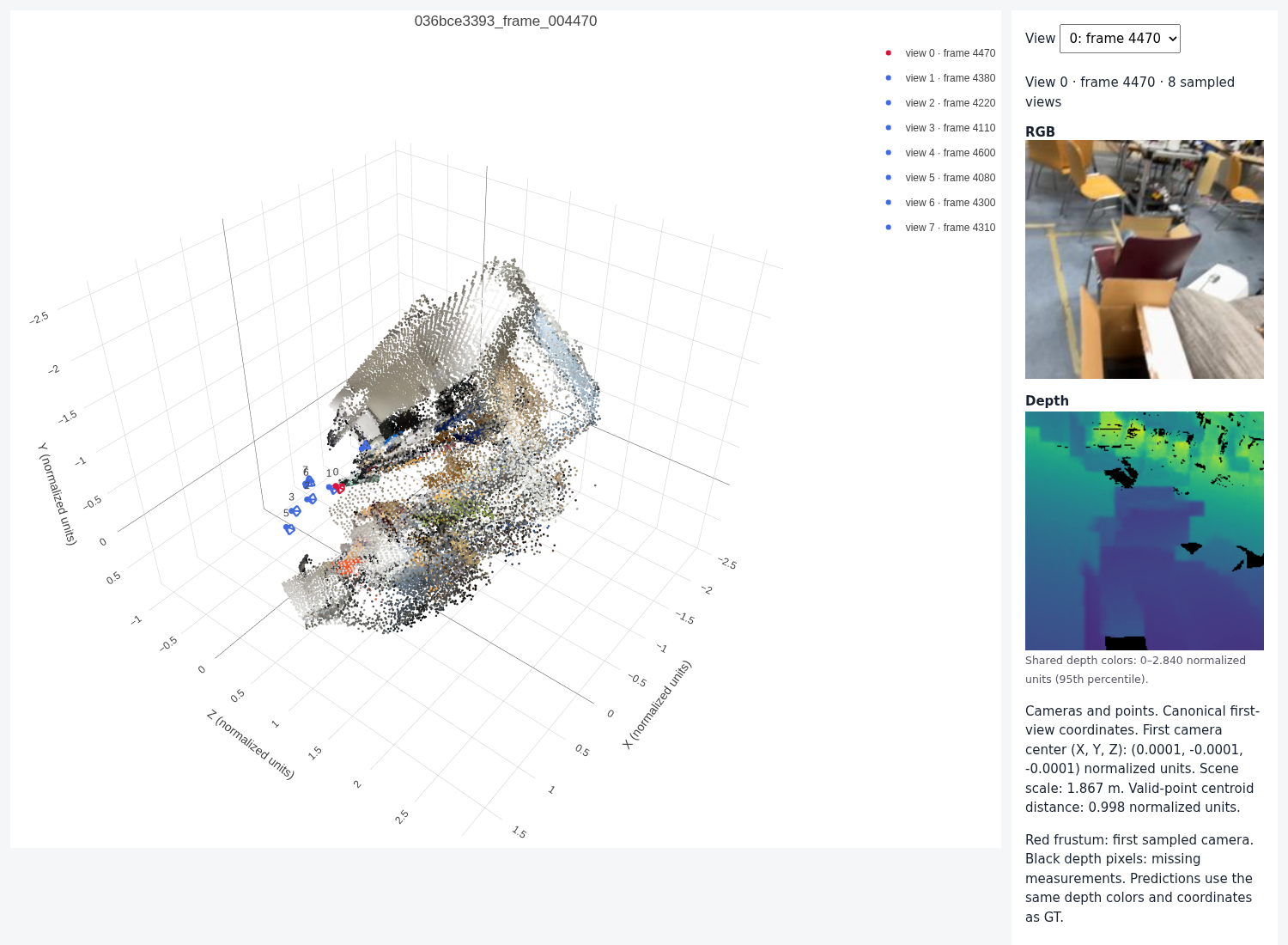
Interactive 3D viewer. The viewer below shows the same overfit clip in 3D. Drag to rotate, scroll to zoom and right-drag to pan. Side by side shows GT and prediction with linked cameras, and Overlay draws both in one frame (GT blue, prediction orange), which makes the small remaining camera and depth errors easy to see. The scene menu also contains the held-out scenes from 3.2. Each cloud has 60,000 of the GT-valid pixels, and the GT and predicted clouds use exactly the same pixels.
Q3.1 overfit clip 036bce3393 (best.pt of the overfit run)
3.2 Training and evaluation (30 points)
Settings. Default model and data settings from configs/vggt.json: frozen DINOv2 ViT-B/14 encoder, 8 frame/global attention pairs (width 384, 6 heads), camera head with 4 blocks, depth head with RGB refinement; 8 views sampled from a 32-frame window, 224×224, global batch size 16 (14 steps per epoch over the 224 training scenes), AdamW with learning rate 6e-4 and weight decay 0.01, 10 warmup epochs, then cosine decay to 5% of the peak, bfloat16, loss weights 5 (camera) and 1 (depth). The only change is the schedule length. The default 1000 epochs would have taken about 8 hours on our shared GPUs, so the run is split into two stages, about 4 hours in total:
- Stage 1 (1 GPU, about 31 s per epoch): the default 1000-epoch schedule, stopped after epoch 265 (2.25 h). At this point the learning rate was still high (5.1e-4).
- Stage 2 (2 GPUs with DDP, the same global batch of 16, about 17 s per epoch): 360 epochs initialized from the stage-1 weights with a fresh optimizer and a fresh 10-epoch warmup + cosine schedule over 360 epochs (1.73 h). This lets the learning rate decay all the way down, which a cut-off 1000-epoch schedule would not.
In total the model sees 625 epochs. best.pt is selected by validation loss: stage-2 epoch 293 (625-epoch scale: 558), with validation loss 0.868.


loss_curve.png of the stage-2 run (epoch 0 is the stage-1 checkpoint) The depth loss drops fast in the first 20 epochs and then flattens, while the camera loss keeps going down slowly for the whole run, so the cameras are the harder and slower part to learn. Restarting the warmup at the start of stage 2 causes no visible jump, and the validation loss falls further once the learning rate decays (from 1.05 at the end of stage 1 to 0.87). The validation loss is lower than the training loss throughout. Training clips are random 8-frame windows of 32 consecutive training frames, while the evaluation clips are fixed and their views are spread over the first 32 prepared frames, so the two losses are not on the same clips.
Metrics (best.pt, 8 views from the first 32 prepared frames, 224 px, seed 825, full splits of 28 scenes each):
| Split | Depth AbsRel ↓ | Depth δ1 ↑ | Rotation AUC @5 / @15 / @30 ↑ | Translation AUC @5 / @15 / @30 ↑ | Joint pose AUC @5 / @15 / @30 ↑ |
|---|---|---|---|---|---|
| Validation | 0.150 | 0.829 | 0.169 / 0.502 / 0.699 | 0.014 / 0.070 / 0.168 | 0.004 / 0.055 / 0.153 |
| Test | 0.172 | 0.758 | 0.190 / 0.492 / 0.699 | 0.005 / 0.040 / 0.136 | 0.000 / 0.026 / 0.120 |
The mean rotation error is 12.4° on validation and 10.3° on test, and the mean translation-direction error is 44.4° and 42.8°. For comparison, the stage-1 checkpoint scored AbsRel 0.180, δ1 0.753 and rotation / translation / joint AUC@30 of 0.584 / 0.131 / 0.110 on validation, so stage 2 improved every metric.
GT vs. prediction on four validation scenes. The left image of each pair is ground truth and the right is the prediction, using the predicted cameras and depth in the same canonical coordinates (red frustum = first camera).


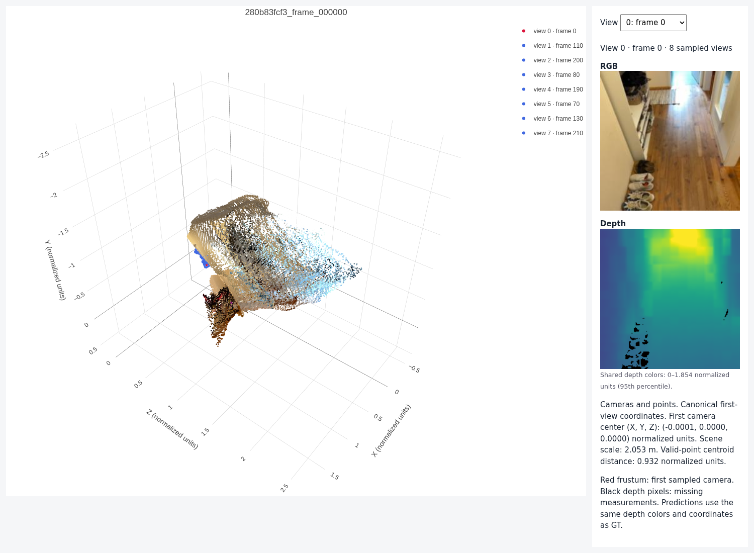


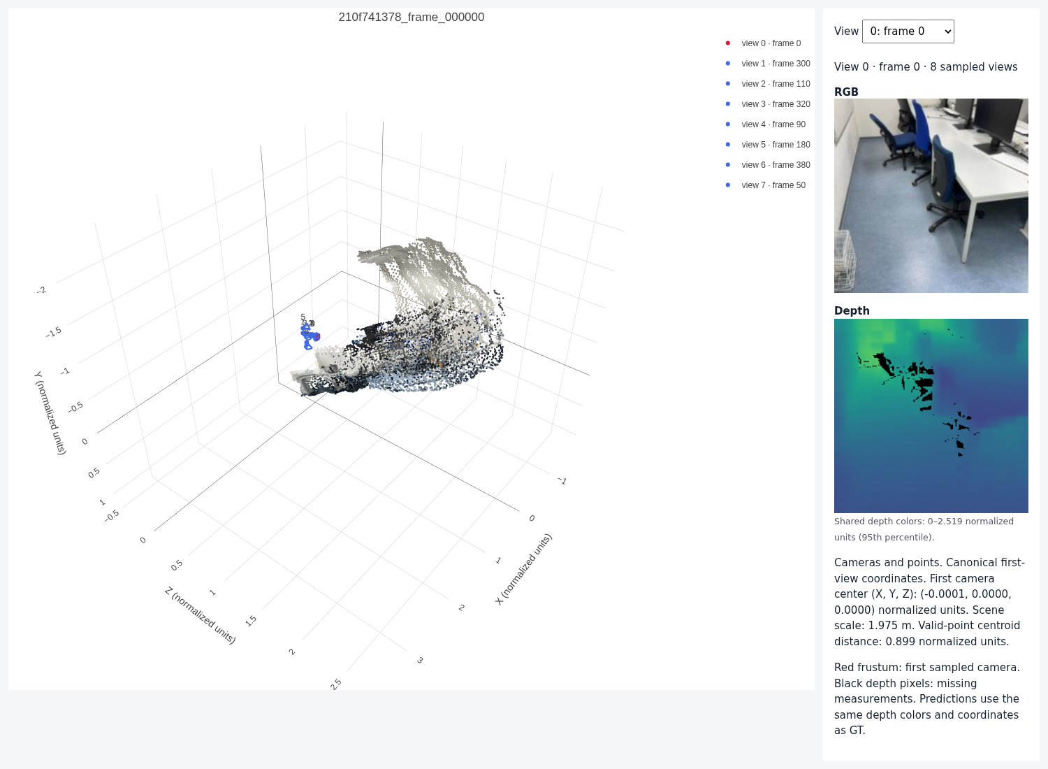
Interactive 3D viewer. All four validation scenes above, plus the four test scenes (including the failure case below), can be explored here from any angle. Pick a scene from the menu and switch between side by side, GT, prediction and overlay. Colour → By view colours each point by the view it came from, which shows how well the 8 per-view depth maps agree with each other.
Q3.2 reconstructions from best.pt (4 validation + 4 test scenes)
Errors on held-out scenes. The model gets the coarse structure of unseen rooms right: floors, walls and large furniture land roughly where they should, the cameras sit in front of the scene facing it, and the scale is close to correct (predicted centroid distances of 0.93–1.08 against the GT value of 1). The errors fall into three groups.
- Depth is over-smoothed. The predicted depth maps keep the large planes but lose thin structures (chair legs, the table edge in the dining room) and show 14×14 blocks, the patch size of the depth head. The point clouds are therefore thicker and blurrier than the GT, and objects bleed into the wall behind them. The depth metrics are decent (δ1 = 0.83 on validation) because most pixels belong to big surfaces, and the errors concentrate at object boundaries.
- Camera translation is the weakest part. Rotation is learned reasonably (AUC@30 ≈ 0.70 on both splits), but the translation direction is not: the mean error is above 40° and AUC@5 is almost 0. In the screenshots the predicted cameras are bunched together more tightly than the GT ones (clearest in the office scene 2b1dc6d6a5, where the GT cameras are spread along a line). A handheld iPhone clip often moves only a few centimetres between frames, so the baseline is a small fraction of the scene and its direction is hard to read from the images. Because the joint pose AUC uses the larger of the two errors, it is limited by translation.
- Large viewpoint changes break the reconstruction. The test scene below has views that look in two very different directions. The GT shows two separate parts of the office, but the prediction squeezes them into one region. When frames overlap little, the global attention has few correspondences to work with, and the model falls back to a prior that the views look at the same thing.
Test scores are a bit lower than validation for depth (AbsRel 0.172 vs. 0.150, δ1 0.758 vs. 0.829), while rotation accuracy is the same, so the gap mostly reflects which scenes ended up in each split rather than overfitting to validation (validation was only used to pick the checkpoint).

3.3 Bonus: number of input views
Question. The model is trained with exactly 8 views. How do accuracy, runtime and memory change if it gets fewer or more views at test time?
Setup. Same best.pt, validation split, first 32 prepared frames, 224 px, seed 825, with V = 2, 4, 8, 16 and 32 views. With a fixed seed, the evaluation loader always picks frame 0 plus the first V − 1 entries of the same random permutation, so the view sets are nested: the 4-view clip contains the 2-view clip, and so on. Runtime and peak memory are for one clip (batch 1, bfloat16, no gradients), averaged over 10 forward passes after 3 warm-up passes. The V = 8 row reproduces the official validation numbers exactly, as a sanity check.

| V | Depth AbsRel ↓ | Depth δ1 ↑ | Rotation AUC@30 ↑ | Translation AUC@30 ↑ | Joint AUC@30 ↑ | Pose pairs | Forward (ms) | Peak memory (GB) |
|---|---|---|---|---|---|---|---|---|
| 2 | 0.116 | 0.871 | 0.683 | 0.164 | 0.125 | 28 | 73* | 0.74 |
| 4 | 0.133 | 0.854 | 0.661 | 0.134 | 0.119 | 168 | 46 | 0.76 |
| 8 | 0.150 | 0.829 | 0.699 | 0.168 | 0.153 | 784 | 47 | 0.80 |
| 16 | 0.183 | 0.780 | 0.669 | 0.148 | 0.129 | 3360 | 52 | 0.89 |
| 32 | 0.191 | 0.750 | 0.654 | 0.142 | 0.125 | 13888 | 184 | 1.05 |
Results.
- Pose is best at the training view count. All three pose AUCs peak at V = 8 and fall off on both sides. With fewer views there is less cross-view context. With more views, the global attention runs over many more tokens than it ever saw in training (32 × 261 instead of 8 × 261), which is a distribution shift. The differences are a few points of AUC, and with V = 2 there is only one pair per scene (28 in total), so the V = 2 pose numbers are noisy.
- Depth gets steadily worse with more views: AbsRel goes from 0.116 to 0.191. Part of this comes from what is being measured. Depth is compared directly in the normalized units (there is no per-image scale alignment), and the normalizing scene scale is computed from the valid points of all V views. The model therefore has to predict every view's depth in a scale shared across the whole clip, and every extra view is one more view whose scale can be off relative to frame 0. With 2 views this only concerns one other frame, while with 32 it concerns 31, and the model never saw clips that long during training. So the drop most likely reflects scale consistency across views and the distribution shift, not that extra views make the per-view depth shape worse.
- Cost. Peak memory grows slowly (0.74 → 1.05 GB), because 0.58 GB of it is the fixed cost of the model weights (144M parameters including the frozen DINOv2), and the activations for a single clip are small. Runtime stays around 50 ms up to 16 views, where the GPU is most likely not yet fully used by one clip, then jumps to 184 ms at 32 views, where the quadratic global attention over 8352 tokens starts to dominate.
Limitations. Only one checkpoint trained with V = 8 and one seed of view sampling were used, and only evaluation was varied (no training with other V). The pose metrics for different V are computed over very different numbers of pairs. Timings were measured on a GPU shared with other jobs, so they are noisy: *the V = 2 time is higher than V = 4, which is noise and not a real effect. Training with a random number of views per batch would be the natural next step to make the model robust to V.
Conclusion. Mini-VGGT works best with the number of views it was trained on. Pose accuracy peaks at V = 8, and both fewer views (less context) and more views (longer global-attention sequences than in training) hurt it. Depth, as measured here, gets steadily worse as V grows, mostly because every view must share one scene scale. The cost of extra views is small up to 16 views (memory is dominated by the weights, runtime stays about flat) and only grows clearly at 32, where the quadratic global attention takes over. To use more views at test time, the model should also see more (or a random number of) views during training.