Assignment 3 for 16-825 (Volume Rendering, NeRF, and 3D Gaussian Splatting)
Experimental setup
- Rays. Ray directions are normalized to unit length, so the sampled depths (
sample_lengths), the segment lengths Δt and the rendered depth are all metric distances along the ray. - Rendering. The transmittance and weights are computed for all samples at once with a single
torch.cumprodalong each ray, instead of a Python loop over the samples. - Sampling. During training,
StratifiedRaysamplerjitters each sample uniformly within its depth bin (stratified sampling). Rendering uses the evenly spaced bin centres. - PSNR. Mean PSNR over the full 128×128 images of a dataset split.
A. Neural Volume Rendering
1.3 Ray sampling (5 points)
get_pixels_from_image maps the pixel indices to the range [-1, 1] in x and y. get_rays_from_pixels appends z = 1 to each pixel coordinate, lifts the points to world space with camera.unproject_points, and sets each ray’s direction to the normalized vector from the camera centre to its lifted point.
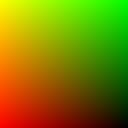
vis_grid)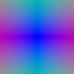
vis_rays)1.4 Point sampling (5 points)
StratifiedRaysampler places n_pts_per_ray depths between min_depth and max_depth. The sample points are origin + depth × direction.
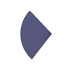
render_points. 1.5 Volume rendering (20 points)
The weight of sample i is Ti(1 − exp(−σiΔti)), where the transmittance Ti = ∏j<i exp(−σjΔtj) and T1 = 1. Color and depth are the weighted sums of the per-sample color and the per-sample depth (sample_lengths).

part_1.gif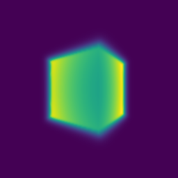
2. Optimizing a basic implicit volume (10 points)
2.1 Random ray sampling. get_random_pixels_from_image draws n_pixels pixels without replacement from the full grid with torch.randperm, on the GPU. 2.2 Loss. Mean squared error between the rendered colors and the ground-truth colors rgb_gt.
After training with train_box:
| x | y | z | |
|---|---|---|---|
| Box center | 0.25 | 0.25 | 0.00 |
| Box side lengths | 2.01 | 1.50 | 1.51 |
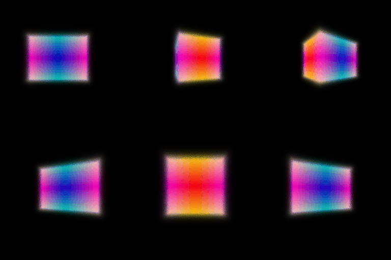
part_2.gif
3. Optimizing a Neural Radiance Field (20 points)
Network. The 3D position goes through a harmonic embedding (6 frequencies) and then an MLP with 6 layers of 128 units and ReLU activations. The embedded input is concatenated again before layer 3 (a skip connection). The last layer outputs 4 values: a ReLU maps the first to density and a sigmoid maps the other three to RGB. Loss. MSE between the rendered and ground-truth colors. Training. The nerf_lego defaults: 250 epochs, 1024 rays per batch, 128 samples per ray, learning rate 5e-4 decayed ×0.8 every 50 epochs.

part_3.gif. PSNR 24.29 on the training views, 23.88 on the test views. 4.1 View dependence (10 bonus points)
Network. As in the NeRF paper, density depends on position only. The 6-layer position MLP outputs a 128-dimensional feature; after a ReLU, a linear layer maps it to density. The feature is concatenated with the harmonic embedding of the normalized ray direction (2 frequencies) and passed through a small color head (one hidden layer of 64 units), which outputs RGB. Training. The nerf_materials settings (250 epochs, learning rate 1e-4) with view_dependence=True. The baseline is the same model with view_dependence=False.


| Materials scene | Train PSNR | Test PSNR |
|---|---|---|
| Without view dependence | 23.26 | 22.75 |
| With view dependence | 23.99 | 23.46 |
Trade-offs. View dependence lets the color change with viewing direction, so the model can represent the specular highlights on the shiny spheres; a model without it can only average them into a dull color. Both train and test PSNR rise by about 0.7 dB, and the gap between them stays the same (about 0.5 dB), so this model does not overfit. The risk grows with how much the network may use the direction. If the direction also fed the density branch, or used many frequencies, the network could explain each training image with view-specific color or geometry instead of one consistent 3D scene, which produces floaters and artifacts at novel views. Keeping density a function of position only, using a low-frequency direction embedding and a small color head limits view dependence to smooth effects such as highlights.
4.2 Coarse/fine sampling (10 bonus points)
Method. Two NeRFs with the architecture from part 3. The coarse network is evaluated at 64 stratified samples per ray. Its rendering weights, normalized, form a piecewise-constant probability distribution along the ray, and inverse-CDF sampling draws 128 extra depths from it. The fine network is evaluated at all 192 depths in sorted order, and its output is the final rendering. Loss. MSE of the coarse rendering + MSE of the fine rendering; the coarse loss keeps the coarse weights a useful sampling distribution. The fine samples are drawn from detached coarse weights. The config is nerf_lego_hierarchical.yaml; the other settings match part 3.

part_4_2.gif (fine network) | Lego | Samples per ray | Train PSNR | Test PSNR | Time per iteration |
|---|---|---|---|---|
| NeRF (part 3) | 128 | 24.29 | 23.88 | 19 ms |
| Coarse/fine | 64 + 128 | 24.56 | 24.19 | 29 ms |
Trade-offs. Coarse/fine sampling gains 0.3 dB of test PSNR. It puts most samples near the surfaces that contribute to the pixel instead of in empty space, which sharpens thin structures such as the bulldozer’s tracks and arm. The cost is a second network (twice the parameters) and about 1.5× the time per training iteration (forward + backward, 1024 rays, measured on one H200). At a fixed compute budget, uniform sampling with more points is a simpler alternative, but its cost grows with the number of samples everywhere on the ray, while importance sampling spends samples only where the coarse network finds content.
4.3 VolSDF (10 bonus points)
Network. A harmonic embedding of the position (6 frequencies) feeds a 6-layer, 128-unit distance MLP that outputs the signed distance (no output activation, since distances can be negative) and a 128-dimensional feature. A 2-layer color MLP maps the feature, after a ReLU, to RGB through a sigmoid. Eikonal loss. The mean of (‖∇d‖ − 1)² at random points in the bounding box; a true signed distance function has unit-norm gradient everywhere. SDF to density. σ(x) = α Ψβ(−d(x)), where Ψβ is the CDF of a zero-mean Laplace distribution with scale β. I write it with exp(−|d|/β), so that neither branch of torch.where can overflow.
Intuition for α and β. α is the density inside the object: far inside the surface σ → α, and on the surface σ = α/2. β controls how sharply the density falls from α to 0 across the surface. The transition has a width of a few β, so a small β gives a nearly solid surface and a large β a soft, foggy one.
- How does high β bias the learned SDF? What about low β? With a high β, density spreads far from the zero level set, so points well outside the object still absorb light. The renderings are blurry, and the learned surface is smoothed, with thin parts thickened or lost. A low β concentrates density at the zero level set, so the model renders a sharp surface close to the true one, but only points very near the surface receive gradient.
- Would an SDF be easier to train with volume rendering and low β or high β? Why? High β. The density, and therefore the gradient, reaches points far from the current surface, so a randomly initialized SDF receives a training signal everywhere along each ray and the surface can move a long way. With a low β, the weights are nearly a delta at the surface, most samples get almost no gradient, and optimization is unstable or stuck early on.
- Would you be more likely to learn an accurate surface with high β or low β? Why? Low β. The renderer then matches opaque surface rendering, and the error-bound argument of VolSDF shows the approximation error shrinks with β. With a high β the photometric loss can be satisfied by a fuzzy shell around the object, so the zero level set does not have to sit on the true surface. In practice one trains with a moderate β first (or learns β) and lowers it.
Experiments. volsdf_surface settings (α = 10, β = 0.05, 250 epochs, learning rate 5e-4), with two eikonal weights:
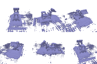

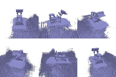

Chosen settings. I keep α = 10 and β = 0.05: β = 0.05 is small compared with the scene (about 1/40 of the bulldozer’s size), so the surface is sharp, yet wide enough that training converges from a random initialization. With eikonal weight 0.02, the color renderings are good, but the extracted mesh has holes and speckles: the field is not a valid SDF away from the surface, so the marching-cubes level set breaks up. Raising the eikonal weight to 0.1 forces a unit-norm gradient everywhere, and the bulldozer becomes a solid, watertight mesh. The remaining clutter around the base comes from the black background, which gives no signal that the space below the bulldozer is empty.
B. 3D Gaussian Splatting
Implementation notes. Each 3D covariance is Σ = R S Sᵀ Rᵀ, built from the quaternion and the scales. It is projected to the image as Σ’ = J W Σ Wᵀ Jᵀ, with W = Rᵀ of the PyTorch3D camera, since PyTorch3D multiplies row vectors (xcam = x R + T). The provided unit test expects W = R, so 2 of its 4 cases fail with my code. I kept Rᵀ because the covariance it gives matches a Monte Carlo estimate (Gaussian samples pushed through the camera), and W = R renders visibly streaky splats. The 2D Gaussian is evaluated as an elementwise quadratic form instead of batched 2×2 matrix products, which is 15× faster with the same output.
5. 3D Gaussian rasterization (35 points)
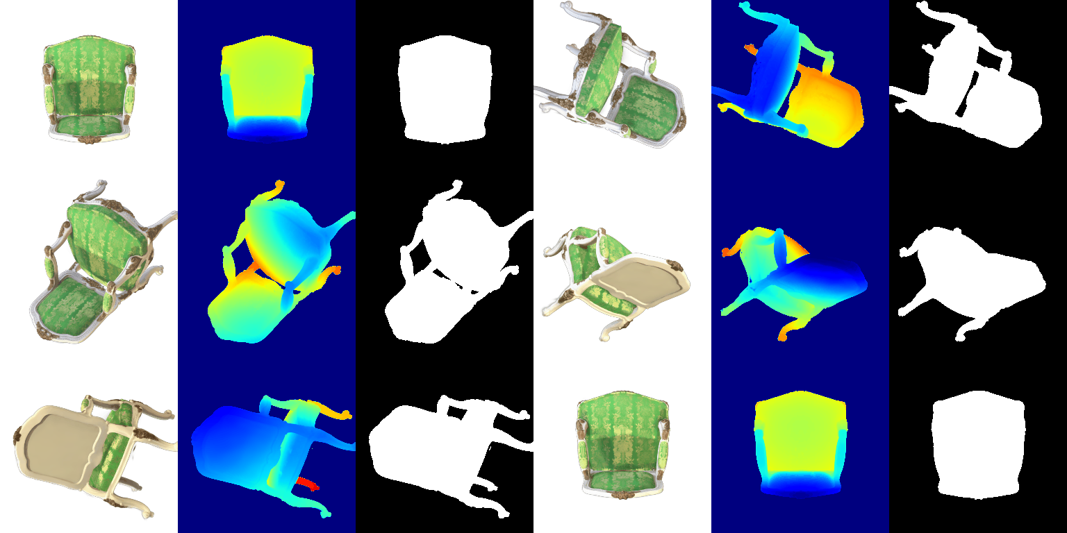
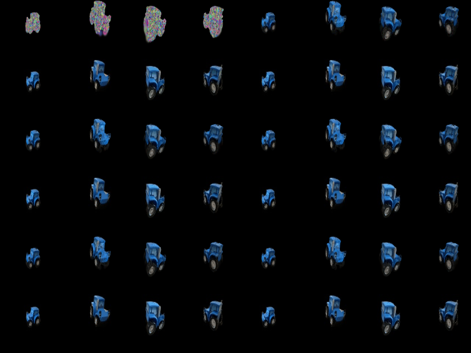
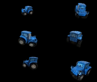
render.py output (DC colour only) 6. Training 3D Gaussian representations (15 points)
Settings. Isotropic Gaussians initialized from the provided points, L1 loss, Adam, 1000 iterations.
| Parameter | Learning rate |
|---|---|
| Opacities | 0.01 |
| Scales | 0.005 |
| Colours | 0.01 |
| Means | 0.0005 |
| Truck (held-out views) | PSNR | SSIM |
|---|---|---|
| Mine | 29.56 | 0.940 |
7.1 Rendering using spherical harmonics (10 points)
Method. The colour of each Gaussian is evaluated from its degree-3 spherical harmonics (16 coefficients per channel) in the direction from the camera centre to the Gaussian mean, plus 0.5, clamped at 0. With only the DC coefficient this reproduces the colours from question 5 exactly.
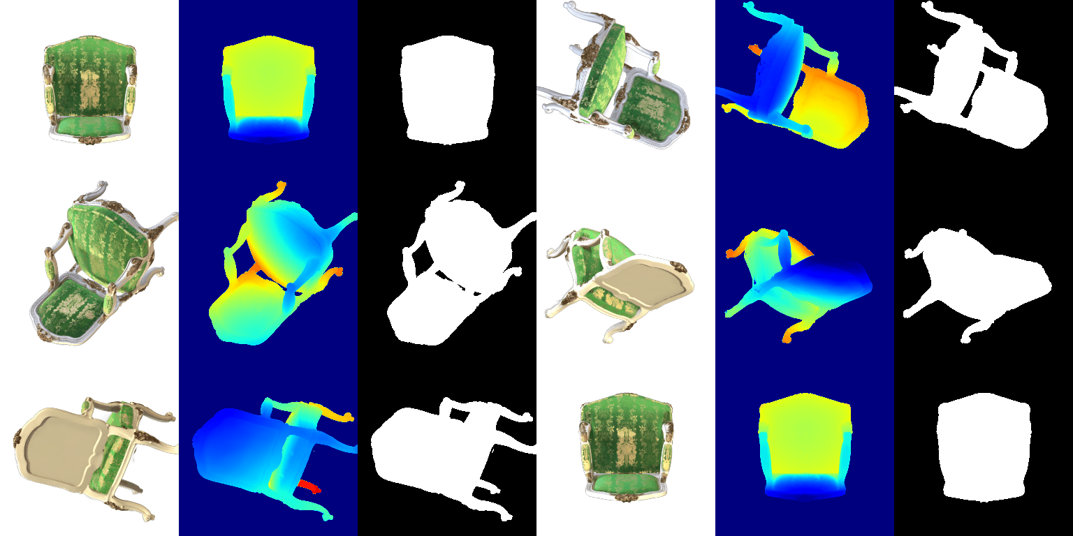
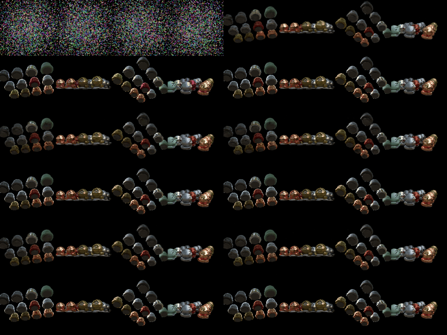
Side-by-side comparisons (left: DC only, right: full SH; same frame):

Frame 4: with SH, the backrest and seat fabric show directional shading: the brocade pattern has brighter highlights and darker folds, while the DC version is flat and uniformly lit. The white frame also gets shading on the side facing away from the view.

Frame 12: the difference is clearest on the seat. Seen from this angle, the SH seat is darker green with glossy gold specular highlights on the pattern, as fabric with a sheen looks from a grazing angle. The DC render keeps the average colour from all views, so it looks lighter and washed out.

Frame 20: from underneath, the two renders are close, since the bottom of the seat is a matte, mostly uniform surface. SH adds slightly stronger contrast on the green side panels and darker shading on the carved wooden parts.
7.2 Training on a harder scene (10 points)
Baseline. The question 6 setup on the materials scene with init_type="random": isotropic Gaussians, the same learning rates, L1 loss, 1000 iterations.
Improved method. Changes relative to question 6:
- Anisotropic Gaussians, with quaternions trained at learning rate 0.001, so a Gaussian can stretch along the spheres’ surfaces.
- Wider random initialization. The means are scaled 5× at initialization, because the materials spheres spread much wider than the default random point cloud, which is concentrated near the origin.
- Loss = 0.8 · L1 + 0.2 · (1 − SSIM), as in the original paper.
- Learning rates. Opacities 0.05, scales 0.005, colours 0.01. The means’ learning rate decays exponentially from 1.6e-3 to 1.6e-5 over training: large steps move the random points into place early, small steps refine them later.
- Simplified adaptive density control. Every 250 iterations from iteration 500 to 3000, Gaussians whose 3D mean has an average gradient norm above 0.0002 are cloned (if small) or split into two smaller ones (if their largest scale exceeds 0.05), and Gaussians with opacity below 0.005 are pruned. The optimizer is rebuilt after each step. This grows the scene from 10,000 to about 49,000 Gaussians.
- Longer training: 6000 iterations.
| Materials (held-out views) | Iterations | PSNR | SSIM |
|---|---|---|---|
| Baseline (Q6 setup) | 1000 | 17.99 | 0.666 |
| Improved | 6000 | 24.47 | 0.897 |
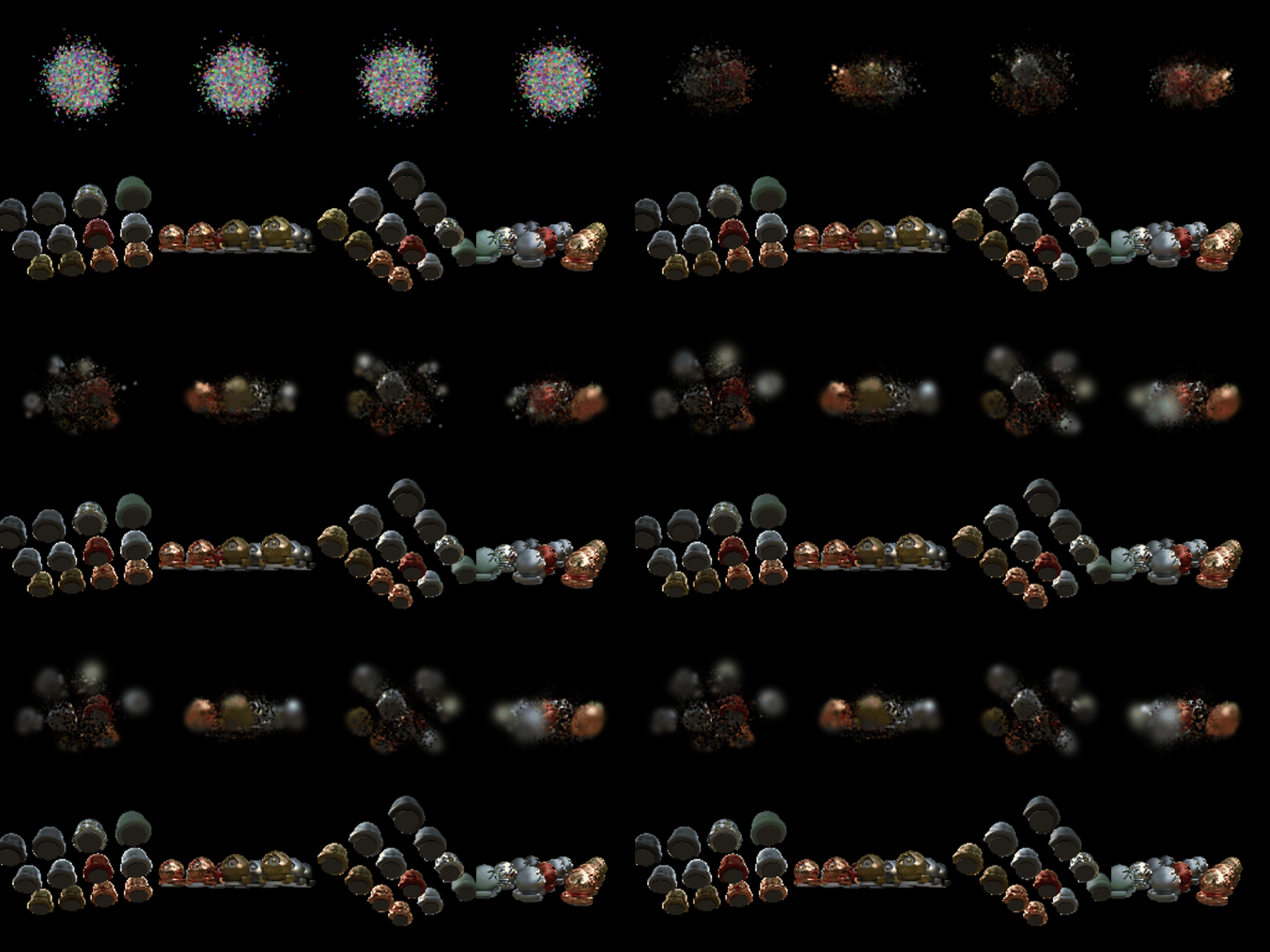
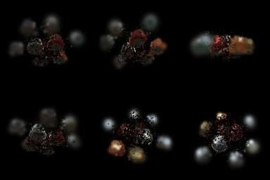
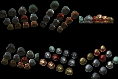
The baseline stays a set of blurry blobs: its isotropic Gaussians start bunched near the origin and the fixed learning rates cannot spread them over all the spheres in 1000 iterations. With the improvements, the individual spheres and their specular highlights are resolved, at +6.5 dB PSNR. Density control contributes most of the detail, since it adds Gaussians exactly where the reconstruction error is largest.