
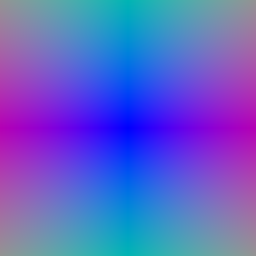
Left: xy grid, right: rays.
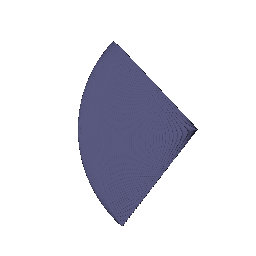
Left: color, right: depth.


Center = (0.25, 0.25, 0.00). Side lengths = (2.00, 1.50, 1.50).


The density depends only on position, but color depends on the viewing direction. Since the direction embedding has fewer frequencies, color can end up varying more slowly with view direction.
128x128. Left: baseline, right: view dependent.


400x400. Left: baseline, middle: view dependent, right: larger view dependent model.


Both small models are blurry, and neither can produce a good shiny/polished sphere, presumable because its appearance changes very quickly with viewing direction. The difference between the baseline and the view dependent model is mostly on the shiny spheres, where the view dependent model changes the brightness with the view. The larger view dependent model is much better, and starts to show some of the reflection on the mirror sphere.
With one color per point, the only way to fit all the training images is the correct geometry, so the multi-view consistency of the images forces the geometry to be correct. If the color can change freely with the direction, it becomes easier to obtain wrong geometry when the camera is far from the cameras that supervised training and still have good renders when the supervised cameras are used - overfitting. View dependence does not make the geometry wrong directly, but allows the network to represent bad geometry more easily since it can hack the loss during optimization.
Alpha is the density inside of the object, and so varying this controls how much light can attenuate along a ray passing through an object. Beta is essentially how "wide" the surface of the object is - how quickly we can transition from being inside the object to outside when traveling normal to its surface.
How does high beta bias your learned SDF? What about low beta?
With high beta, the render can be blurry because the boundary of the object is "stretched" across space, normal
to the actual surface. This can also cause thin parts to disappear completely or break. With low beta, the surface is sharper,
but this also makes optimization harder since the probably of sampling a point exactly in this region is lower, and so the gradients
are more sparse.
Would an SDF be easier to train with volume rendering and low beta or high beta? Why?
Higher beta is easier to optimize, since the chances of getting a sample in the diffuse region of the boundary is more.
Would you be more likely to learn an accurate surface with high beta or low beta? Why?
Lower beta produces more accurate surfaces, though there is still a bias near the object's actual surface. Since the region
representing the boundary is both thinner and closer to the actual surface of the object, the representation is more accurate.
Best result:
Eikonal weight = 0.1, alpha = 10, beta = 0.05, num epochs = 250, learning rate = 5e-4, MLP: 6 layers, 128 units,
Softplus (beta = 100) (from the IDR paper), 6 frequencies.


The default eikonal weight of 0.02 leaves a large flat surface underneath the model. My hypothesis is that due to there not
being enough variation in camera positions to supervise this region below the model, it doesn't end up getting pinned by the
color loss. A larger eikonal weight removes this.


Beta. All with eikonal weight 0.1 and alpha = 10.
The best result was with beta = 0.05. I also tried a few other values:
beta = 0.2:
The renderer gets enough density from regions where the SDF comes close to 0 but stays positive. So
thin parts can appear in the render with no zero crossing, and marching cubes loses them. Its possible that a different
threshold for marching cubes can recover some of this detail, but this affects the whole model and may end up inflating it.


beta = 0.01:
The hypothesis here is as above - with small beta values, there isn't enough signal to actually learn the model.


These were attempted without varying the alpha values. The original paper mentions that they set alpha to the reciprocal of beta,
so as to attenuate the light that gets past an object as its boundary becomes more diffuse. Setting a rule for alpha based on beta, and then scheduling
beta from coarse to fine may make it easier to learn and produce high quality renders, at the cost of training time.

Note: when computing the 2D covariance, using camera.R makes the unit tests pass, but using camera.R.transpose(-1, -2) produces better outputs and reconciles there difference between the PyTorch3D and 3DGS conventions (and so I use the transposed version).
I trained for 1000 iterations. The learning rates are as follows:
PSNR: 30.26, SSIM: 0.946.
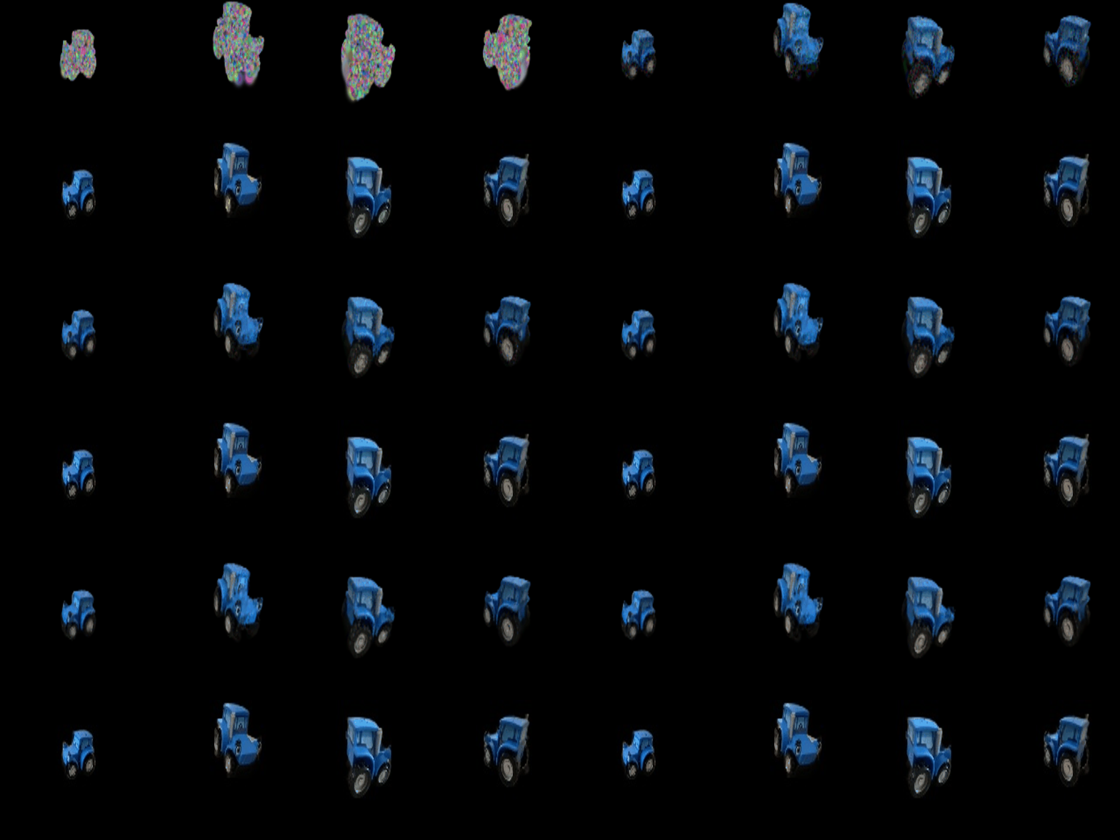

DC spherical harmonics (from question 5.5)
All spherical harmonics

Frame 4. Left: DC SH, right: All SH.

Frame 12. Left: DC SH, right: All SH.

Frame 20. Left: DC SH, right: All SH.
