Assignment 3
Neural Volume Rendering and 3D Gaussian Splatting
Contents
A. Neural Volume Rendering
1.3. Ray Sampling
5 pointsPixel coordinates are generated on a W × H grid and mapped to NDC in [-1, 1]. Each NDC point is placed on the image plane at z = 1 and unprojected to world space with camera.unproject_points. Ray origins are the camera center, broadcast to every pixel. Ray directions are the normalized vectors from the origin to the unprojected points.
rays_o = camera.get_camera_center().expand(N, 3)
rays_d = normalize(unproject(xy_ndc, z=1) - rays_o)

vis_grid)
vis_rays)1.4. Point Sampling
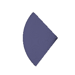
5 pointsStratifiedRaysampler places n_pts_per_ray evenly spaced depths between min_depth and max_depth. Each sample point is the ray origin plus that depth times the ray direction. The figure shows the sample points of the first camera as a point cloud.
z = linspace(near, far, n_pts)            # (n_pts, 1)
points = origins[:, None] + z * directions[:, None]   # (B, n_pts, 3)
1.5. Volume Rendering
20 pointsTransmittance is an exclusive cumulative product of exp(−σ Δt) along each ray, so T = 1 for the first segment. The weight of each sample is T · (1 − exp(−σ Δt)). Color and depth are weighted sums of the sample colors and sample depths. The depth map is normalized by its maximum value.
T_i = Π_{j<i} exp(−σ_j Δt_j)
w_i = T_i · (1 − exp(−σ_i Δt_i))
C = Σ_i w_i · c_i        D = Σ_i w_i · t_i
part_1.gif)
2. Optimizing a Basic Implicit Volume
10 points2.1 Random ray sampling. Each iteration draws a random permutation of all pixel indices and keeps the first batch_size. The same pixel subset is used to generate rays and to sample ground-truth colors from the image.
2.2 Loss. Mean squared error between rendered colors and rgb_gt.
| Parameter | Value after training (rounded to 0.01) |
|---|---|
| Box center | (0.25, 0.25, 0.00) |
| Box side lengths | (2.01, 1.50, 1.50) |
2.3 Visualization. My spiral rendering of the optimized box (left) matches the TA reference (right).

part_2.gif)
3. Optimizing a Neural Radiance Field (NeRF)
20 pointsSample positions are encoded with HarmonicEmbedding using 6 frequencies, which gives 39 dimensions. The encoding goes through a 6-layer MLP with 128 hidden units and ReLU. The encoded input is concatenated again before layer 3 as a skip connection. The final layer outputs 4 values. The first goes through ReLU to give density, and the other three go through Sigmoid to give RGB. The loss is MSE on randomly sampled rays (1024 per iteration). I trained with the default nerf_lego.yaml settings: 250 epochs, 128×128 images, 128 samples per ray, learning rate 5e-4.
x → γ(x) [39] → MLP(6 × 128, skip @ layer 3) → [σ_raw, rgb_raw]
σ = ReLU(σ_raw),  rgb = Sigmoid(rgb_raw)

part_3.gif)4.1. View Dependence
Bonus · 10 pointsI follow the NeRF design. The xyz trunk outputs a 128-d feature instead of colors. Density comes only from that feature through a linear head and ReLU, so geometry cannot depend on the viewing direction. Color comes from a small branch: the feature is passed through a linear layer, concatenated with the harmonic encoding of the ray direction, and then fed to Linear(128+15 → 64) → ReLU → Linear(64 → 3) → Sigmoid. The direction is broadcast to every sample on its ray.
h = ReLU(MLP_xyz(γ(x)))
σ = ReLU(W_σ h)
rgb = Sigmoid(MLP_dir([W_f h, γ_dir(d)]))
All runs below use nerf_materials.yaml (250 epochs, lr 1e-4, 128 samples per ray). Only the view-dependence setting changes between them.


nerf_materials_highres.yamlObservations. Without view dependence (a), each point has a single color, so the specular highlights on the spheres are averaged into the diffuse color. The spheres look flat and blotchy. With a low-frequency direction encoding (b, d), the highlights on the white and teal spheres change smoothly as the camera moves, and the surfaces look cleaner. With 8 direction frequencies (c), the surfaces become noisier and speckled, even though the color branch can fit the training views more closely.
Trade-off between view dependence and generalization. More view dependence lets the model represent non-Lambertian effects such as specularities and reflections. However, it also gives the network a shortcut: it can explain each training image with direction-specific colors instead of learning correct geometry and a consistent appearance (the shape–radiance ambiguity). The training loss then goes down while novel views get worse, with floaters, flickering highlights, and noisy textures. These effects become more visible when the training views are sparse. I limit this capacity in three ways: (1) density never sees the direction; (2) the direction enters only a shallow, narrow branch near the output; (3) the direction encoding uses only a few low frequencies, which keeps color a smooth function of direction. Setting (b) gave the best balance. Raising the direction frequencies, as in (c), moves toward overfitting.
B. 3D Gaussian Splatting
5. 3D Gaussian Rasterization
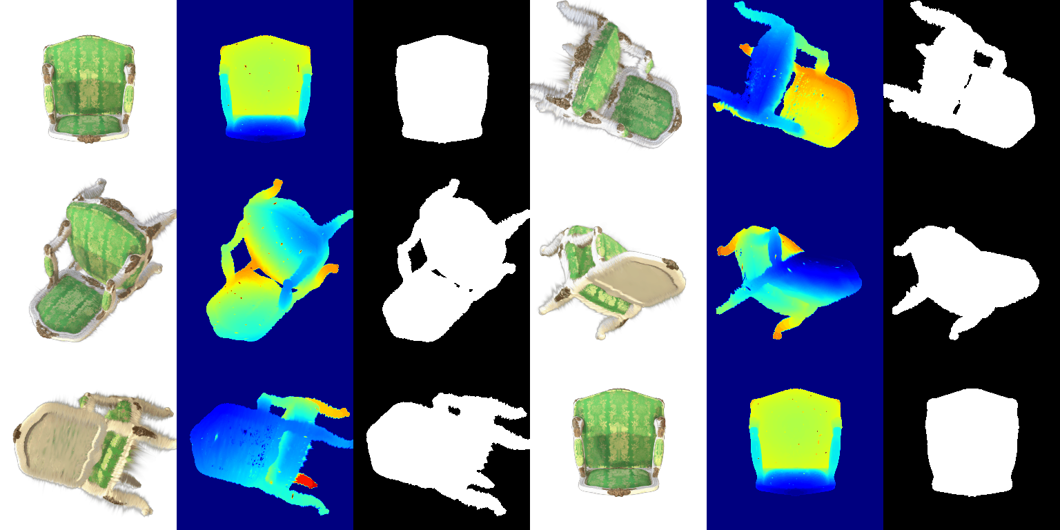
35 pointsThe 3D Gaussians are projected to 2D using Σ' = J W Σ Wᵀ Jᵀ with Σ = R S Sᵀ Rᵀ. They are filtered and sorted by depth, then alpha-composited front to back with α = opacity · exp(power) and an exclusive cumulative product for transmittance. All 4 unit tests pass. The GIF below comes from render.py with the pre-trained chair Gaussians, showing RGB, depth, and silhouette.
part_5_render.gif)6. Training 3D Gaussian Representations
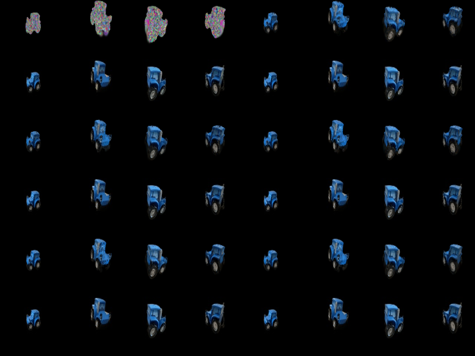
15 pointsIsotropic Gaussians are initialized from the truck point cloud and trained with an L1 loss between the rendered and ground-truth images, on a black background. I use Adam with a separate learning rate for each parameter. The means get the smallest rate so the geometry from initialization stays stable, while opacities and colours can change faster.
| Setting | Value |
|---|---|
| Learning rate · opacities | 0.05 |
| Learning rate · scales | 0.005 |
| Learning rate · colours | 0.02 |
| Learning rate · means | 0.0005 |
| Loss | L1 |
| Iterations | 1000 |
| Mean PSNR (held-out views) | 29.823 |
| Mean SSIM (held-out views) | 0.942 |

7.1. Rendering Using Spherical Harmonics
10 pointsEach Gaussian's 48 SH coefficients (16 basis functions × RGB, degree 3) are evaluated in the direction from the camera center to the Gaussian mean. The result is offset by 0.5 and clamped at 0, which reproduces the reference get_color in vectorized form. With all non-DC coefficients set to zero, the output matches the DC-only colours of Q5.5 exactly.
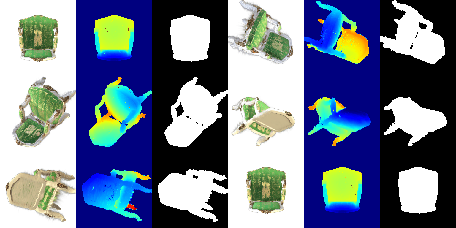
Side-by-side comparisons (left: DC only · right: full SH)

Facing the backrest, the DC-only render has a bright, washed-out green, and the gold pattern is low contrast. With SH, the fabric is a deeper green and the gold brocade stands out clearly. The wood on the armrests also has more pronounced highlights and shadows. The DC term stores an average color over all viewing directions, while the higher-order terms restore how the shiny brocade and carved frame look from this particular direction.

This view shows the same effect. With SH, the seat cushion is darker than the backrest, matching how differently oriented fabric reflects light toward the camera. In the DC version, both surfaces have nearly the same flat brightness. The gold decorations on the frame look metallic only with SH.

From above, the SH render shows view-dependent shading on the seat and backrest, with darker regions where the fabric faces away from the camera. The difference is smaller than in the front views, because the DC color is closer to the true appearance for this direction. The geometry, depth, and silhouette are identical in both renders, since SH only changes the color. This frame matches the README reference with SH: mean RGB difference 0.41/255, compared with 5.62/255 against the reference without SH.