Assignment 2: Single View to 3D
Fitting geometric representations, learning single-image reconstruction, and exploring an implicit occupancy decoder.
Setup and evaluation
This submission covers 1.1–1.3, 2.1–2.5 and option 3.1. The optional extensions 3.2 and 3.3 are not included.
The chair-only R2N2/ShapeNet split contains 6,100 training objects and 678 test objects. All learned models use RGB input with an ImageNet-pretrained ResNet18, trained end-to-end on an NVIDIA A100. Cached ResNet features were not used.
All main results below use the final 30,000-step checkpoints, not a mixture of the best test scores from different runs. Adam uses a batch size of 32 and seed 0. The learning rate is 0.0004 through step 20,000 and 0.0001 for steps 20,000–30,000. Training was resumed between stages with Adam state preserved.
Evaluation covers all 678 test objects, using one randomly selected view per object with seed 0. F1 is calculated per object using nearest-neighbor Euclidean distances and averaged over objects; scores are on a 0–100 scale. The baseline evaluation uses 1,000 sampled points; the 2,000-point experiment also changes the evaluation sampling count.
For voxel and implicit outputs, probabilities are converted to meshes at threshold 0.5. The starter evaluation applies a 180° Y rotation and separate centering of predicted and target points. Point and mesh evaluation do not apply that extra centering. The GIFs use shared framing without independently rescaling the prediction and GT.
1. Exploring loss functions
1.1. Fitting a voxel grid
4 pointsThe voxel parameters are logits optimized directly with binary cross-entropy with logits. This combines the sigmoid and BCE in a numerically stable operation.
L = mean(softplus(s) − y · s)
Occupied voxel locations are rendered as points. This is fitting one object, not generalization from an unseen RGB image.

1.2. Fitting a point cloud
3 pointsThe Chamfer loss is implemented as two nearest-neighbor queries with knn_points. It sums the mean squared distance from each predicted point to the target and from each target point to the prediction.
L = mean_x min_y ||x − y||² + mean_y min_x ||y − x||²
The reverse direction encourages coverage of the target, while the forward direction discourages outlying predictions. The implementation does not call the packaged Chamfer loss.

1.3. Fitting a mesh
3 pointsVertex offsets deform an icosphere. Surface-sampled Chamfer loss fits the shape, and uniform Laplacian smoothing penalizes deviations from neighboring vertices. The objective is:
L = L_chamfer + 0.1 · L_laplacian
Smoothing discourages irregular local geometry, but does not guarantee that the mesh is free of self-intersections.

2. Reconstructing 3D from a single view
2.1. Image to voxel grid
20 pointsA linear layer maps the 512-dimensional image feature to a 512×2×2×2 tensor. Four 3D transposed convolutions upsample it to 32³ occupancy logits. The training loss is BCEWithLogitsLoss.


The model captures bulky chair structure, but thin frames remain incomplete and some surfaces merge. The coarse grid limits fine detail.
2.2. Image to point cloud
20 pointsAn MLP with dimensions 512 → 512 → 1024 → 3N predicts N=1,000 points. Training uses the bidirectional squared Chamfer loss defined in 1.2.


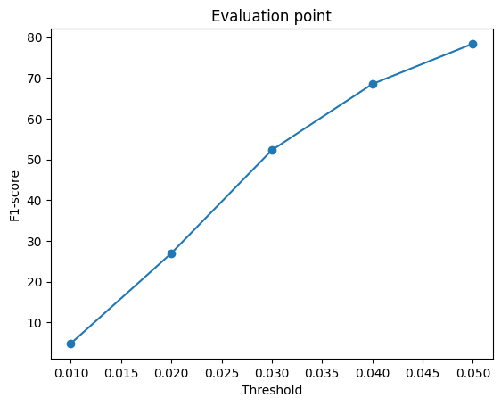
The prediction can distribute points over separate chair parts without fixed connectivity. The renderings remain sparse, and a good distance score does not imply a watertight surface.
2.3. Image to mesh
20 pointsAn MLP predicts vertex offsets from a level-4 icosphere scaled by 0.5. Surface Chamfer has weight 1.0 and Laplacian smoothing has weight 0.1.


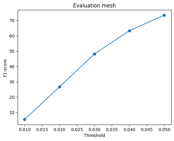
Connected surfaces are produced, but folds and merged structures can remain. A deformed sphere cannot freely change its connectivity to match chair holes and disconnected parts.
Comparing representations
| Model | F1@0.01 | F1@0.03 | F1@0.05 ↑ |
|---|---|---|---|
| vox | 4.708 | 46.167 | 74.515 |
| point | 4.856 | 52.268 | 78.386 |
| mesh | 5.528 | 48.094 | 73.369 |

Among the three baseline representations, points have the highest F1@0.05. Voxels slightly exceed meshes at this threshold. Point placement is unconstrained by grid resolution or template connectivity, which can help surface coverage. Voxels retain coarse structure but lose thin details; meshes provide surfaces but can distort when matching complex topology. These are possible explanations, not isolated causal findings. The extra voxel centering is also a difference in evaluation protocol.
2.4. Hyperparameter experiments
10 pointsNumber of predicted points
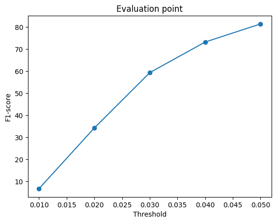
The main comparison changes N from 1,000 to 2,000 while holding the training step budget, learning-rate schedule, batch size, encoder and seed fixed.
| Model | F1@0.01 | F1@0.03 | F1@0.05 ↑ |
|---|---|---|---|
| point | 4.856 | 52.268 | 78.386 |
| point_n2000 | 6.749 | 59.293 | 81.349 |
At 30,000 steps, 2,000 points improve F1@0.05 by 2.963 percentage points. The denser output can improve surface coverage, but also increases output-layer parameters. The same option increases target sampling density during training and evaluation, so this is a combined change rather than a pure resolution ablation. Only one seed was used.


Training duration and reduced learning rate
| Model | 10,000 steps | 20,000 steps | 30,000 steps |
|---|---|---|---|
| vox | 61.350 | 68.432 | 74.515 |
| point | 79.125 | 79.225 | 78.386 |
| mesh | 72.724 | 73.257 | 73.369 |
| point_n2000 | 84.585 | 82.861 | 81.349 |
| implicit | 43.239 | 59.934 | 70.536 |

Voxel and implicit models benefit from additional training. Point-cloud scores peak earlier and then decrease; the mesh changes only modestly. Lower training loss therefore does not imply higher test F1. The 30,000-step stage also lowers the learning rate, so its effect cannot be separated from the extra training steps. Without a held-out validation study, this does not establish overfitting as the cause. All stages are disclosed, and the main gallery consistently uses the final stage rather than selecting checkpoints by test score.
2.5. Interpreting the model
10 pointsDivide the RGB image into a 4×4 grid and replace one patch at a time with ImageNet mean RGB (0.485, 0.456, 0.406). Compare each prediction to the unoccluded prediction. Brighter regions indicate larger output changes.
- Voxels: mean absolute occupancy-probability change.
- Points: bidirectional squared Chamfer between outputs.
- Meshes: mean displacement of corresponding vertices.
Vox


Point


Mesh


These maps show how local image perturbations affect the entire reconstructed shape, complementing the final output visualizations. A high response identifies sensitivity to that patch, not necessarily evidence used correctly. Inspect the color bar of each map separately: the representations use different change measures and their values cannot be compared directly.
Occlusion may introduce unnatural inputs; the grid is coarse, and the measurement tracks prediction change rather than accuracy. Thus it is a sensitivity experiment, not causal attribution.
3. Exploring other architectures
3.1. Implicit occupancy network
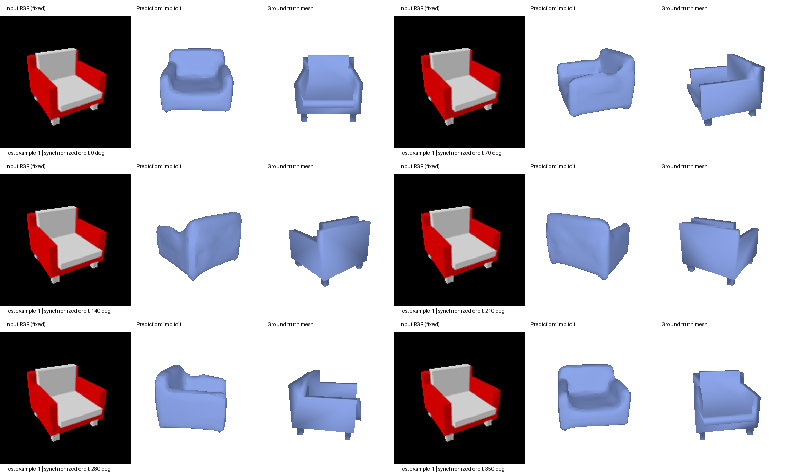
10 pointsThe decoder predicts occupancy at a query location conditioned on the image feature: f(z_image, x, y, z). The 512-dimensional image feature and the 3D coordinate are projected into 128 dimensions and added. This is equivalent to a first affine layer on their concatenation. ReLU and two 128-unit hidden layers lead to a scalar occupancy logit.
image feature + query coordinate → MLP → occupancy logit
32 × 32 × 32 queries → occupancy grid → marching cubes
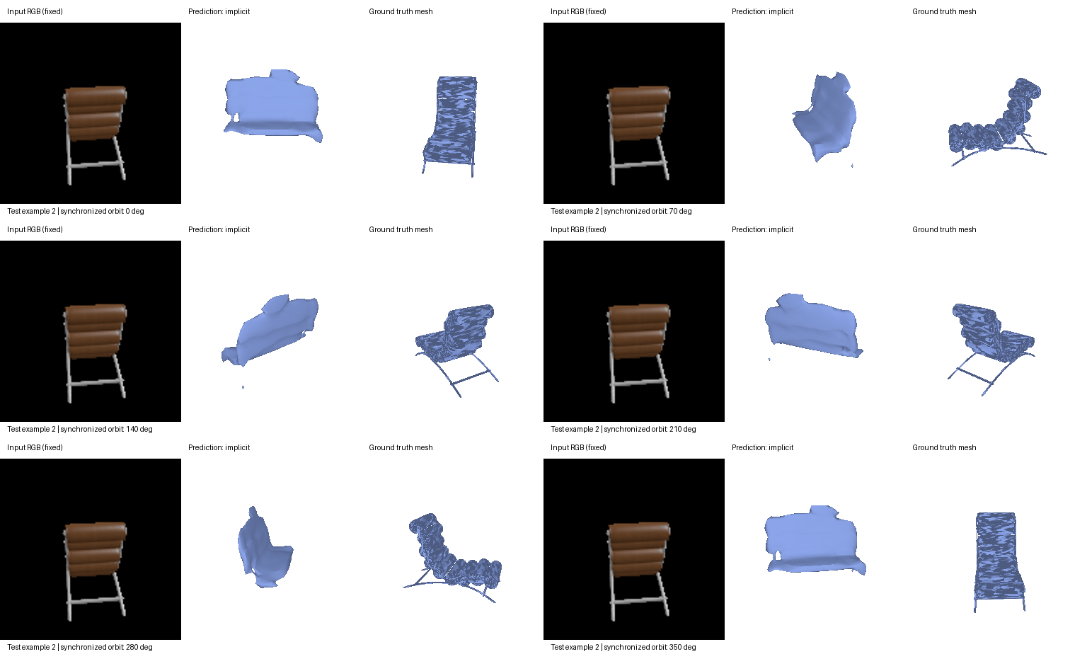
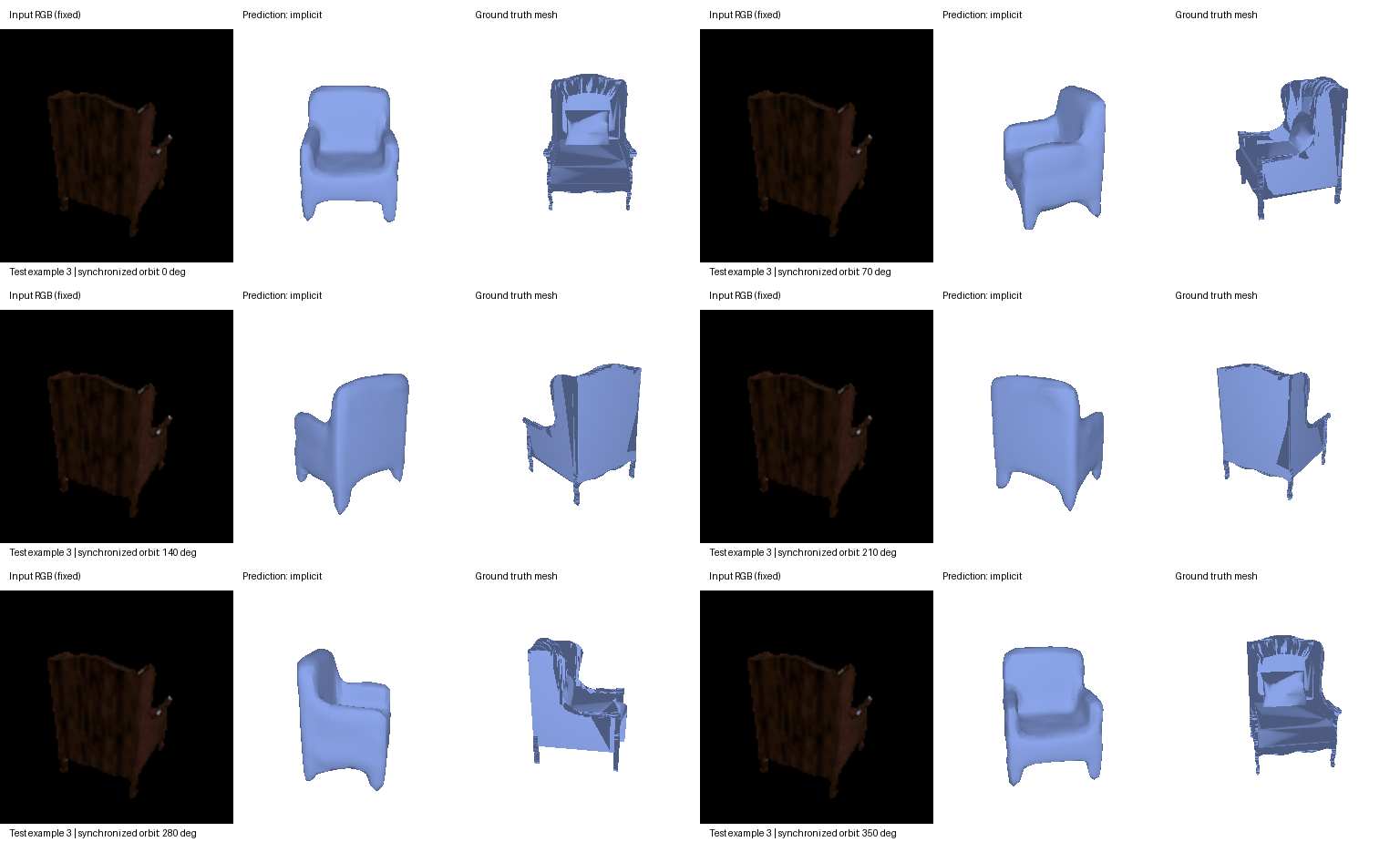
Queries are arranged in Z,Y,X grid order while each coordinate vector is (x,y,z). To match the existing voxel labels, the normalized coordinate is 2i/32 − 1 for i=0,…,31, giving [-1, 0.9375] inside the normalized cube. All 32³ locations are supervised with BCE; arbitrary coordinates can also be queried. The labels are the assignment’s surface-voxel occupancy, not an independently computed solid interior occupancy field.
| Model | F1@0.01 | F1@0.03 | F1@0.05 ↑ |
|---|---|---|---|
| vox | 4.708 | 46.167 | 74.515 |
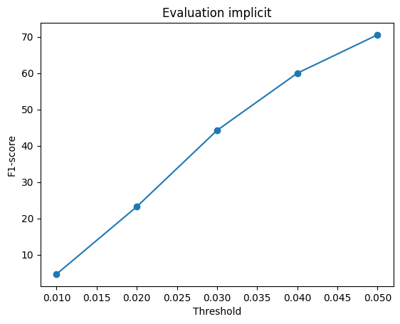
| implicit | 4.635 | 44.215 | 70.536 |
The implicit model improves from 43.239 at 10,000 steps to 70.536, but remains 3.980 points below the final voxel decoder. Conditioning a coordinate MLP on global image features provides a continuous query function, but does not by itself guarantee fine geometry or better accuracy. Thin chair structures remain difficult under the coarse surface-voxel supervision.
Measurements and reproducibility
All images are stored in the local assets folder. GIFs contain synchronized prediction/target views. Click any image to open it at full size.
- vox: metrics and evaluation settings
- point: metrics and evaluation settings
- mesh: metrics and evaluation settings
- point_n2000: metrics and evaluation settings
- implicit: metrics and evaluation settings
- Checkpoint training settings
- All three training-stage scores
- Asset provenance
The single-object fitting tensors do not record their training-step counts, so no exact fitting duration is claimed for section 1. Sections 2 and 3 use checkpoint-verified step counts.