1. Differentiable volume rendering
1.3. Camera rays
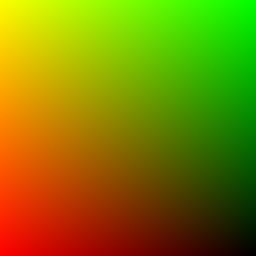
Pixel locations are mapped into normalized device coordinates. Unprojecting those coordinates gives a point on each camera ray; subtracting the camera center and normalizing gives its world-space direction.
1.4. Sampling points along a ray
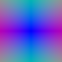
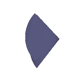
Each sample position is the ray origin plus its distance times the unit ray direction. Sampling remains inside the configured near and far bounds.
1.5. Emission–absorption rendering
A segment with density σ and length Δ has opacity α = 1 − exp(−σΔ). Its transmittance is the product of (1 − α) over earlier segments, so the first segment has transmittance one. The renderer sums RGB values weighted by αT. Replacing RGB by sample distance gives the depth map.


2. Optimizing a basic implicit volume
Random pixel subsets limit memory during training. Mean squared RGB error updates the box center and side lengths from the four supplied posed views.
| Parameter | Result |
|---|---|
| Center (x, y, z) | (0.25, 0.25, 0.00) |
| Side lengths (x, y, z) | (2.01, 1.50, 1.50) |
| Epochs / updates | 1000 / 4000 |
| Final training MSE | 0.0000009 |
| Training time (minutes) | 0.35 |

The optimized box is wider along x and displaced toward positive x and y. Its orbit retains the colored faces of the supplied target. The rendered edges remain soft because the SDF-to-opacity mapping uses a finite-width transition.
3. Optimizing a neural radiance field
The MLP encodes 3D position with sine and cosine features. Its density branch uses ReLU and its color branch uses sigmoid. Training minimizes RGB mean squared error on sampled rays from the supplied Lego training split. The checkpoint selected by validation PSNR is evaluated on held-out test images. This experiment uses position-dependent color.
| Model | Test PSNR (dB) | Test SSIM | Epochs | Selected epoch | Updates | Training (min) | Test rendering (s) | Parameters |
|---|---|---|---|---|---|---|---|---|
| Uniform sampling | 24.17 | 0.8812 | 250 | 250 | 25,000 | 2.95 | 4.72 | 101,252 |
| Coarse + fine | 24.49 | 0.8881 | 250 | 250 | 25,000 | 3.74 | 7.91 | 202,504 |


The orbit reconstructs the yellow bulldozer body, raised arm, tracks, and gray base from front, rear, and side views. At 128-pixel resolution, track edges, windows, and small mechanical parts remain soft, and the arm has a few irregular edges.
The supplied split contains 100 training, 100 validation, and 200 test views. Both runs use seed 1, 128 × 128 images, and batches of 1,024 rays.
PSNR is computed from image RGB error; SSIM compares local image structure. The reported values are means over held-out views. Baseline configuration and full measured results record the run settings.
4.2. Coarse/fine sampling
The coarse network first estimates density along each ray. Its rendering weights define a probability distribution for additional samples. Inverse-CDF sampling places more points in intervals that contribute to the rendered color. A separate fine network evaluates the combined, depth-sorted sample locations. Both networks receive RGB supervision. The baseline queries 128 uniform samples. The hierarchical model queries 64 coarse locations, adds 64 importance samples, and evaluates the fine network at all 128 sorted locations: 192 network queries per ray in total.


The coarse/fine orbit keeps the same bulldozer layout and resolves some small edges more distinctly. The gain is modest: studs and the underside remain smooth, and dark spots persist beneath the platform. Importance sampling improves the measured reconstruction without removing every visible artifact.

Relative to the baseline, coarse/fine sampling changes test PSNR by +0.31 dB and SSIM by +0.0068. Measured optimization time is 1.27× the baseline; held-out rendering time is 1.68×. These are measurements from the recorded runs on the same desktop, including their stated configurations and epoch counts. The GPU was shared with Gaussian training and other desktop workloads during part of these runs. These wall times are observations under that load, not a controlled or equal-compute speed benchmark. Training timings exclude validation and final rendering.
Concentrating samples near occupied regions can resolve detail that uniform sampling misses. The second network and its extra evaluations cost memory and time. Early coarse predictions can also direct samples poorly, so retaining uniform samples gives the fine network coverage of the whole ray. Coarse/fine configuration.
5. 3D Gaussian rasterization
Each Gaussian covariance is constructed from its scale and rotation. A perspective-projection Jacobian maps the covariance into image space. Gaussians behind the camera are discarded; the remainder are sorted front to back. Their projected Gaussian power, opacity, and accumulated transmittance determine each pixel contribution. The same weights accumulate color, depth, and silhouette.

6. Training a Gaussian representation
The supplied truck point cloud initializes the centers of isotropic Gaussians. Training updates centers, scales, opacities, and RGB colors through the differentiable renderer using L1 image loss. Held-out camera views are reserved for evaluation.
| Setting / metric | Value |
|---|---|
| Iterations | 1000 |
| Gaussians | 10000 |
| Seed | 3 |
| Training time (minutes) | 5.18 |
| Held-out views | 5 |
| Mean test PSNR (dB) | 29.35 |
| Mean test SSIM | 0.9398 |
| Parameter | Learning rate |
|---|---|
| opacities | 0.05 |
| scales | 0.005 |
| colours | 0.01 |
| means | 0.0001 |


7.1. Rendering with spherical harmonics
The pretrained chair includes spherical harmonic coefficients. Evaluating their directional basis at each camera-to-Gaussian direction produces view-dependent RGB values. The DC-only baseline and the full spherical harmonic render use the same geometry, opacity, camera poses, and rasterizer.


The paired images isolate the effect of the directional color coefficients. No held-out ground-truth images are supplied for this chair, so a visible difference alone does not establish a quantitative accuracy improvement.
Reproduction and checks
| Environment | Version / device |
|---|---|
| device | NVIDIA GeForce RTX 5090 |
| python | 3.11.16 |
| torch | 2.8.0+cu128 |
| cuda | 12.8 |
| pytorch3d | 0.7.9 |
The implementation, training, evaluation, rendering, report figures, and archive generation ran on the desktop. The report verifier decodes every GIF frame, checks all local links and required outputs, and verifies finite metrics. The Gaussian projection regression checks three rotated anisotropic cases against autograd and finite-difference Jacobians. Renderer checks cover mini-batch equivalence, finite gradients, and DC-only spherical harmonic agreement. The unchanged supplied fixtures pass two of four cases: the two cases that depend on projected covariance encode the opposite rotation convention. PyTorch3D uses X_cam = X_world R + T for row vectors, so the covariance transform uses W = Rᵀ. The chair renders use this corrected convention.
python build_report.py
python verify_artifacts.py
python package_submission.py
Setup and complete commands · Environment · Measured results · Artifact verification
Starter code, datasets, and assignment instructions: learning3d/assignment3. The NeRF implementation follows the sampling procedure described by Mildenhall et al. Gaussian projection and compositing follow Kerbl et al. The spherical harmonic basis follows the reference linked in the assignment. These implementation references are separate from the experiments reported above.