1. Exploring loss functions
1.1. Fitting a voxel grid
Binary cross entropy compares the predicted logits with binary occupancy targets. A sigmoid converts logits to probabilities for visualization. Direct fitting uses Adam with a learning rate of 0.05; decoder training uses 0.0004.

The optimized grid matches the target silhouette in the front and side views. The coarse grid makes the chair’s thin frame thicker than the original mesh.
1.2. Fitting a point cloud
Chamfer loss adds the mean squared nearest-neighbor distance in each direction. The implementation uses knn_points for the searches and computes the reduction explicitly. Fitting uses 5,000 points.

The points move into the seat, back, and lower frame. Sampling remains uneven, with clusters along edges and a few stray points visible in the side view.
1.3. Fitting a mesh
The mesh starts as a level-4 icosphere with radius 0.35. Chamfer loss compares sampled surface points, while uniform Laplacian smoothing penalizes the distance from each vertex to its neighbors’ average. The smoothing weight is 0.1.

The back and seat approach the target, but stretched triangles fill much of the space below the seat. The fixed sphere topology makes the open lower frame difficult to reproduce.
2. Reconstructing 3D from a single view
The chair split contains 5,490 training objects, 610 validation objects, and 678 test objects. Validation holds out 10% of the supplied training objects. Training samples an available RGB view; evaluation uses each object’s lowest available test view. All models use the same test inputs and ground-truth sampling seeds.
The encoder is ImageNet-pretrained ResNet18, trained with the decoder. All runs use RGB inputs; cached ResNet features are disabled. Adam starts at 0.0004 with batch size 32 and seed 7. Validation runs every 2,000 steps. Training stops after five evaluations without improvement, once 10,000 steps have passed, or at 100,000 steps. The checkpoint with the highest validation F1@0.05 is evaluated.
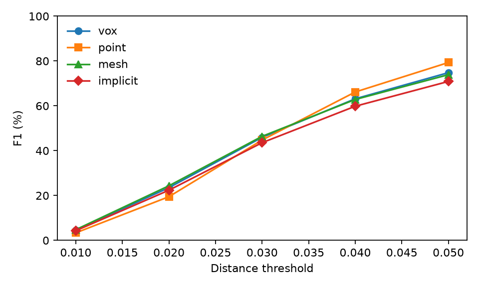
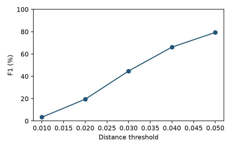
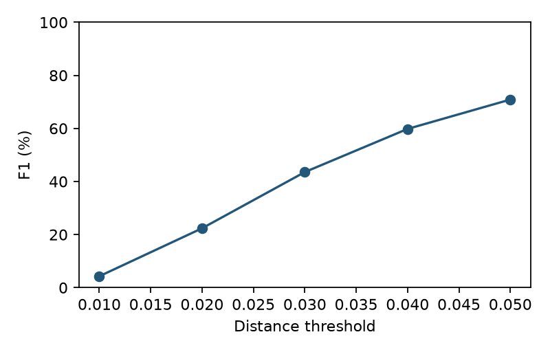
F1 is the harmonic mean of surface precision and recall, reported as a percentage. Each reconstruction is compared with 1,000 points sampled from the ground-truth mesh. The threshold is Euclidean distance in the starter’s coordinate system. Voxel predictions retain the starter’s half-turn around y and sample-centering convention; point and mesh predictions use their direct coordinates. Empty extracted surfaces receive F1 = 0.
| Representation | Test F1@0.05 (%) | Selected step | Training steps |
|---|---|---|---|
| vox | 74.79 | 46,000 | 56,000 |
| point | 79.32 | 4,000 | 14,000 |
| mesh | 73.89 | 4,000 | 14,001 |
2.1. Image to voxel grid
A linear layer maps the 512-dimensional image feature to a 4³ feature volume. Three transposed 3D convolutions produce 32³ occupancy logits. Marching cubes extracts the probability-0.5 surface.
Test F1@0.05 is 74.79%. The examples use the first, middle, and last object in the supplied test ordering, shared across all models.

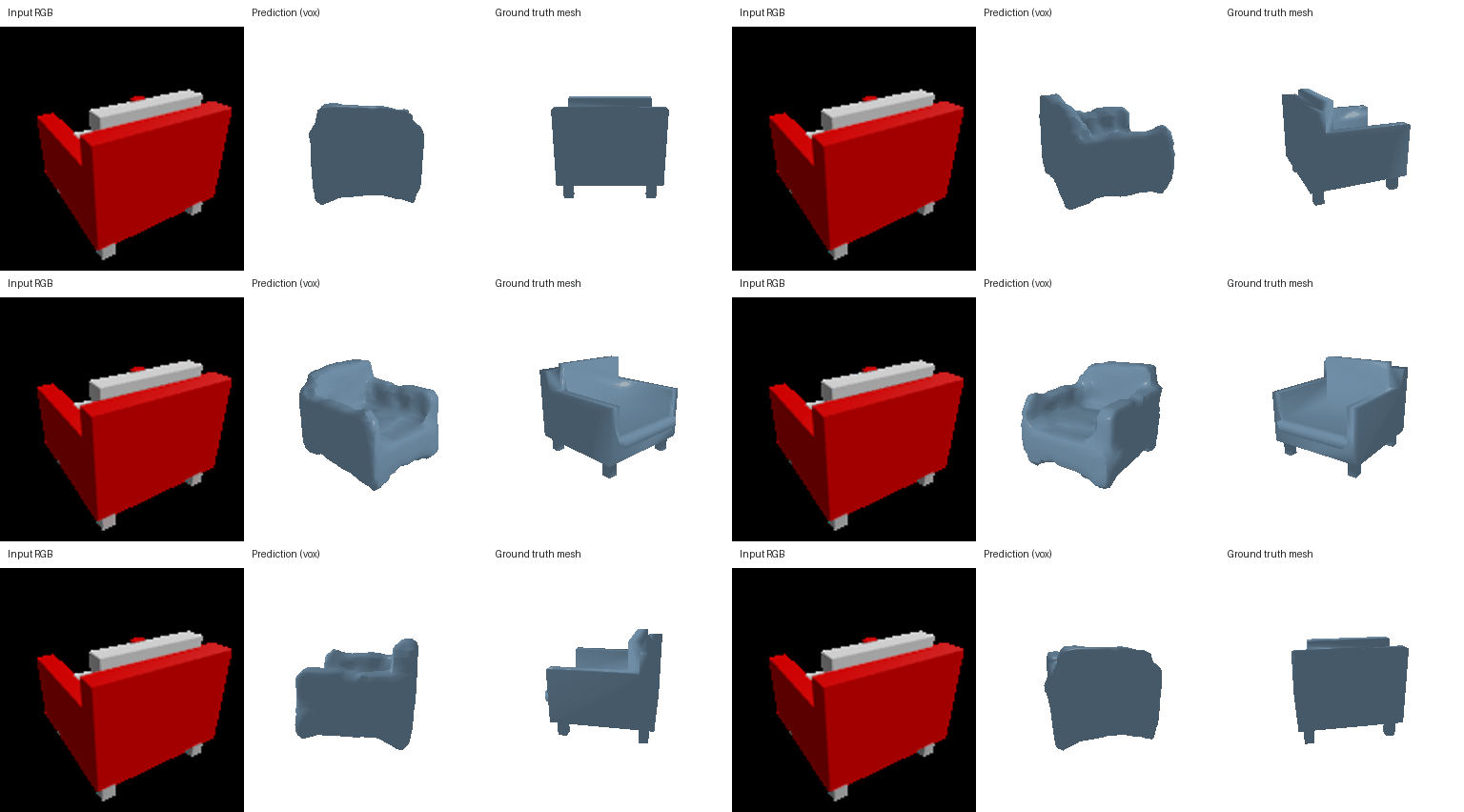
c04660caf4670baed40fb6f8053555de, view 00. F1@0.05: 81.35%.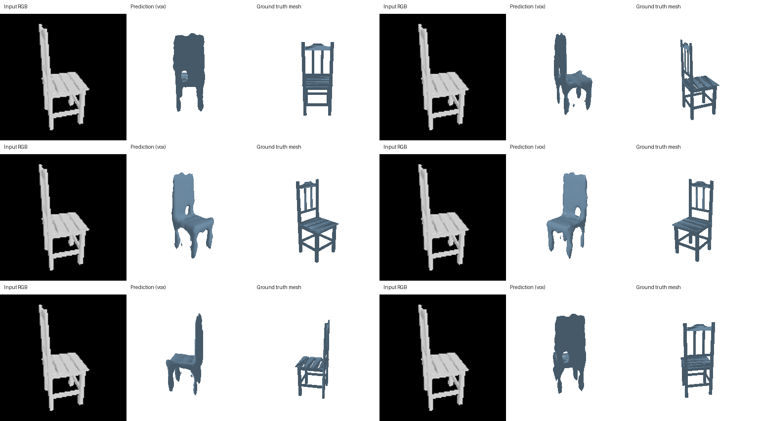
768ea32d8303095bfe6f9308e75765b1, view 00. F1@0.05: 82.44%.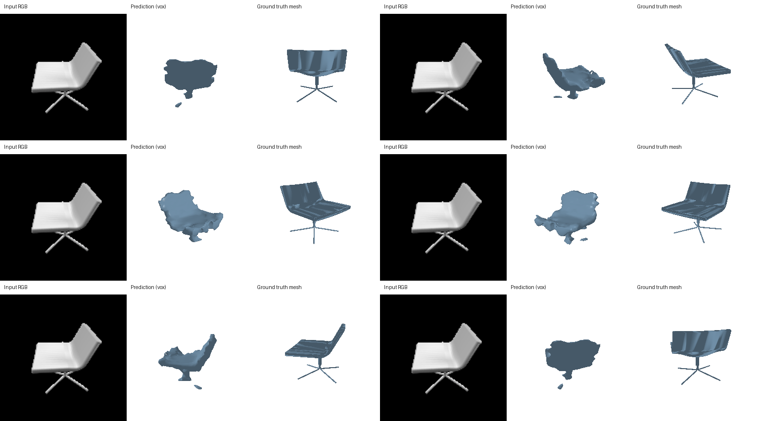
37235898ebd06b3b504721639e19f609, view 00. F1@0.05: 94.98%.
7dc902a12843fa60e84c9243a4e577f, view 00.The first two examples retain the seat and back, but narrow slats merge into broad surfaces. The pedestal chair’s thin base is mostly missing. In the lowest-scoring bench example, the prediction contains only small fragments and loses most of the back and legs.
2.2. Image to point cloud
The point decoder is an MLP with two 1,024-unit hidden layers. Its output is reshaped into 1,000 xyz points. Training compares these points with a deterministic 10,000-point surface pool, using a new random subset each step.
Test F1@0.05 is 79.32%. The examples use the first, middle, and last object in the supplied test ordering, shared across all models.
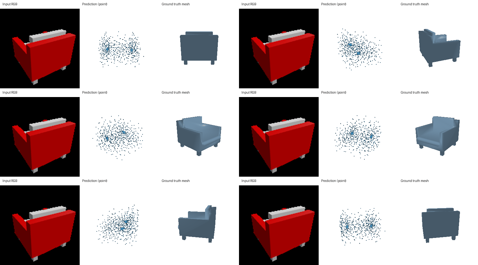
c04660caf4670baed40fb6f8053555de, view 00. F1@0.05: 64.16%.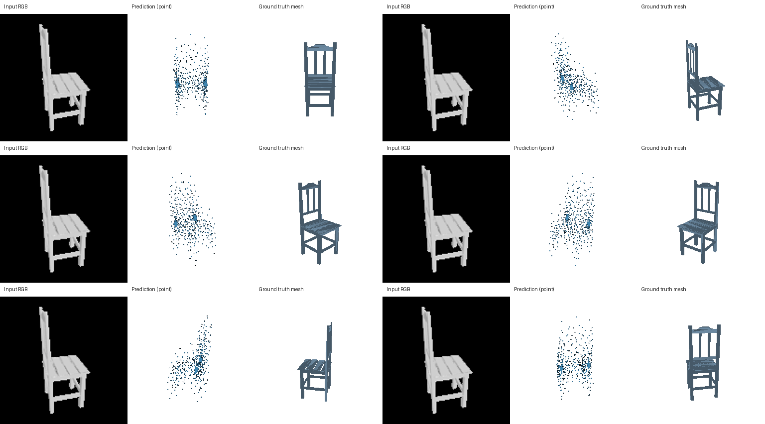
768ea32d8303095bfe6f9308e75765b1, view 00. F1@0.05: 92.36%.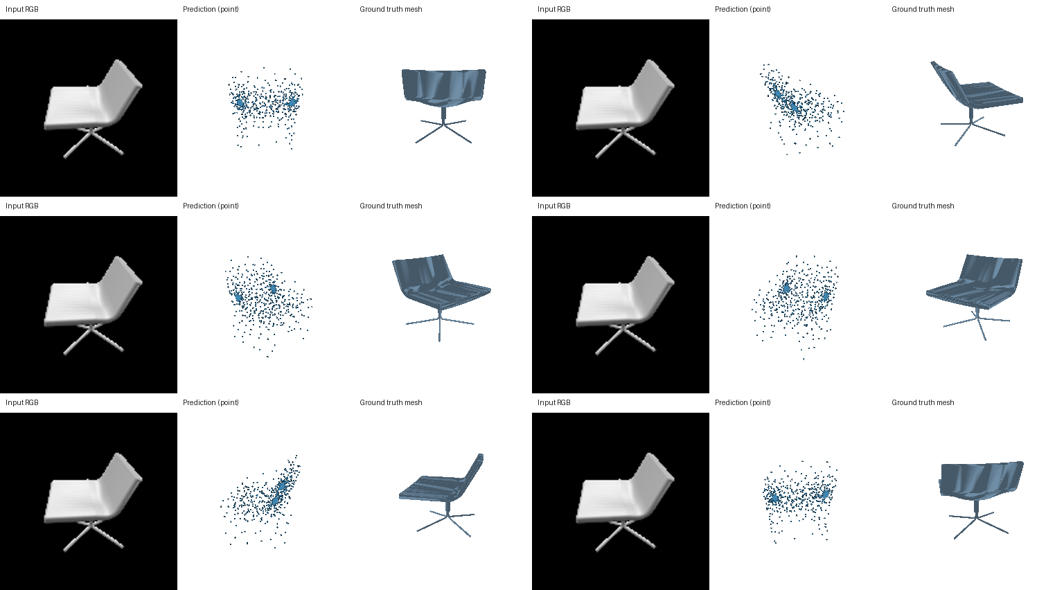
37235898ebd06b3b504721639e19f609, view 00. F1@0.05: 73.43%.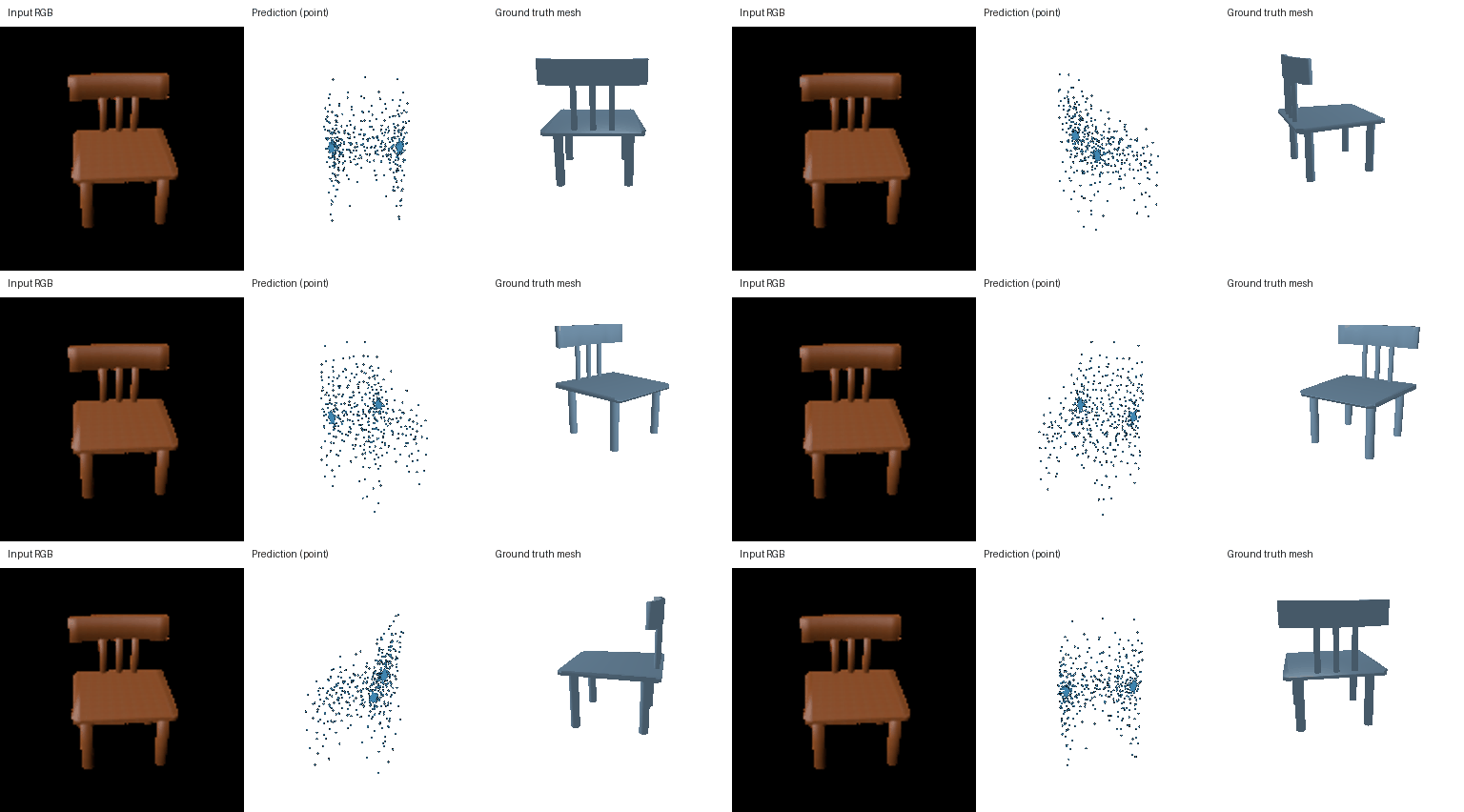
6730fb4ca7c90ddccd8b2a7439d99cc3, view 00.The points roughly trace the backs and seats, but the clouds are diffuse and thin frame members are poorly separated. In the lowest-scoring wooden-chair example, the broad backrest is replaced by scattered points and the legs lose their straight structure. A higher mean F1 does not make this a clean surface representation.
2.3. Image to mesh
The mesh decoder predicts offsets for the 2,562 vertices of a level-4 icosphere. Triangle connectivity stays fixed. The final layer starts at zero, so the first prediction is the undeformed sphere. Each step samples its predicted surface and compares it with a random subset of the same 10,000-point target pool used by the point model.
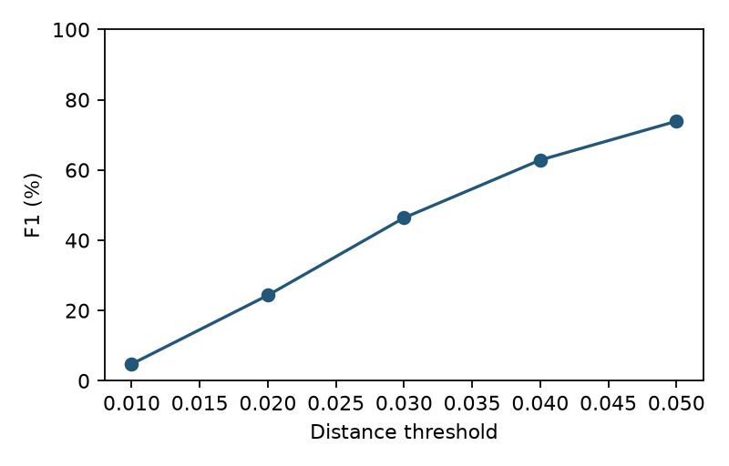
Test F1@0.05 is 73.89%. The examples use the first, middle, and last object in the supplied test ordering, shared across all models.
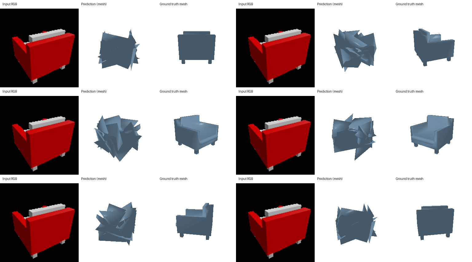
c04660caf4670baed40fb6f8053555de, view 00. F1@0.05: 74.31%.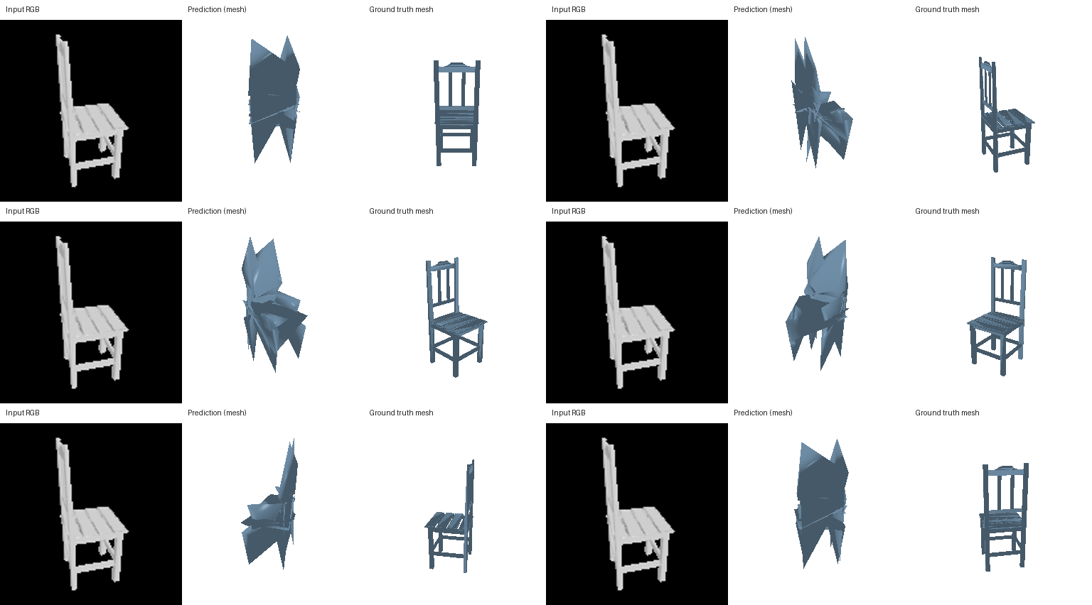
768ea32d8303095bfe6f9308e75765b1, view 00. F1@0.05: 84.23%.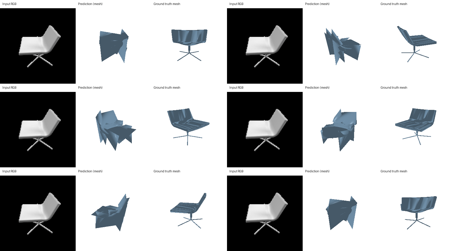
37235898ebd06b3b504721639e19f609, view 00. F1@0.05: 49.00%.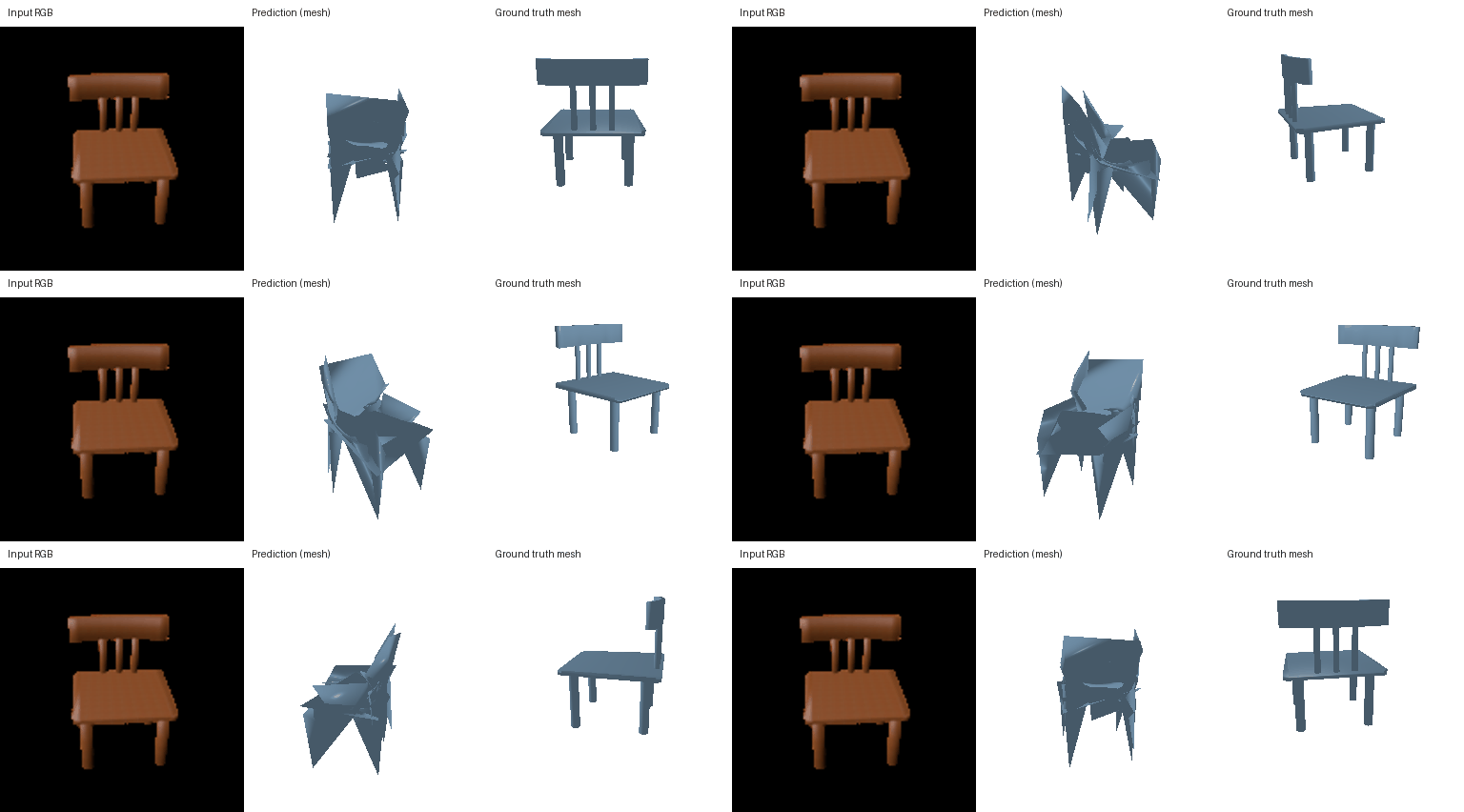
6730fb4ca7c90ddccd8b2a7439d99cc3, view 00.The baseline follows the broad seat/back layout, but its triangles fold across the open frame. In the wooden-chair failure, it creates a broad sheet where the target has separate back supports, with long spikes below the seat. Surface samples can be close to the chair even when triangle connectivity looks poor.
The measured ordering is point (79.32%), vox (74.79%), then mesh (73.89%). Point outputs can put samples on disconnected chair parts, but do not define a continuous surface. Voxels have a fixed spatial resolution. The mesh is continuous, but its sphere connectivity restricts which openings and disconnected parts it can represent. These constraints help interpret the renders; training and checkpoint selection also affect the scores.
2.4. Mesh smoothing weight
The three mesh runs differ only in smoothing weight. They use the same initialization, data split, seed, learning rate, batch size, and stopping rule. Each selects its own best validation checkpoint.
| Smoothing weight | Test F1@0.05 (%) | Validation F1@0.05 (%) | Selected step |
|---|---|---|---|
| 0 | 74.69 | 74.15 | 14,000 |
| 0.1 | 73.89 | 73.05 | 4,000 |
| 1 | 72.25 | 70.73 | 26,000 |

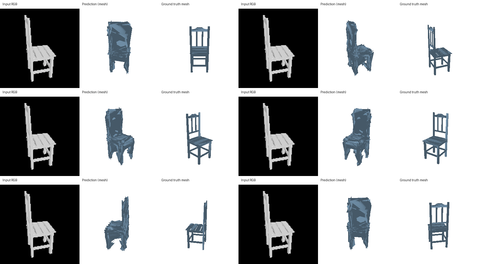
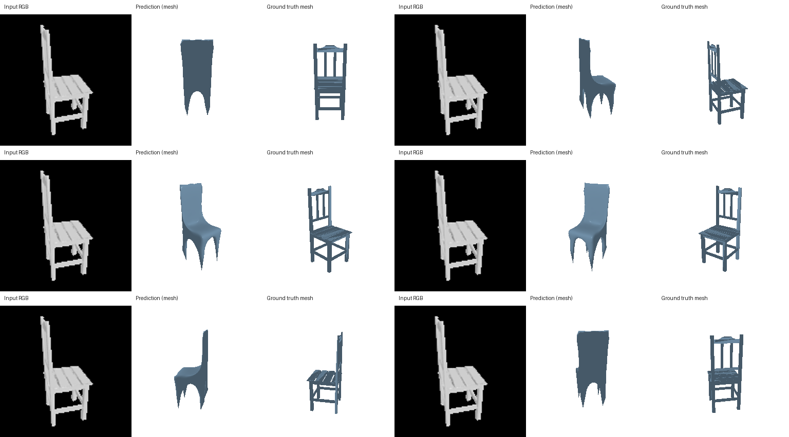
Weight 0 gives the highest test F1 in this comparison (74.69%). Relative to weight 0.1, removing smoothing changes F1 by +0.80 percentage points; raising the weight to 1 changes it by -1.64 points. The comparison uses each run’s validation-selected checkpoint. F1 measures surface proximity, so the turntables are also needed to judge triangle quality and whether the open frame is retained. With weight 0, the shared chair has many small folds. Weight 1 produces a smoother silhouette, but fills the open back and lower frame. The small F1 advantage of weight 0 comes with visibly rougher geometry.
2.5. Which image regions affect the point prediction?
For each of the three point-model examples, a 4×4 grid divides the input into 16 patches. Each patch is replaced by the ImageNet mean color, then the model predicts another point cloud. The heatmap shows squared bidirectional Chamfer distance from the original prediction. It measures sensitivity to this occlusion procedure; it does not establish which pixels are necessary for recognition.


The largest changes for the three chairs are 0.00104, 0.00114, and 0.00131 in squared Chamfer distance. In the second example, hiding the lower-right patch spreads the lower-frame points farther apart and shifts part of the cloud to the right. The reconstruction changes beyond the masked image region, so this decoder does not treat each patch as an independent 3D part.
3.1. Implicit occupancy decoder
The implicit decoder combines a 128-dimensional projection of the image feature with an xyz query. Hidden layers of 256, 256, and 128 units predict an occupancy logit. Query coordinates span [−1,1]³ in voxel-index order. Each training step uses 2,048 uniformly sampled grid locations. Evaluation queries all 32³ locations in chunks and extracts a surface at probability 0.5.
| Decoder | Test F1@0.05 (%) | Selected step |
|---|---|---|
| vox | 74.79 | 46,000 |
| implicit | 70.89 | 30,000 |
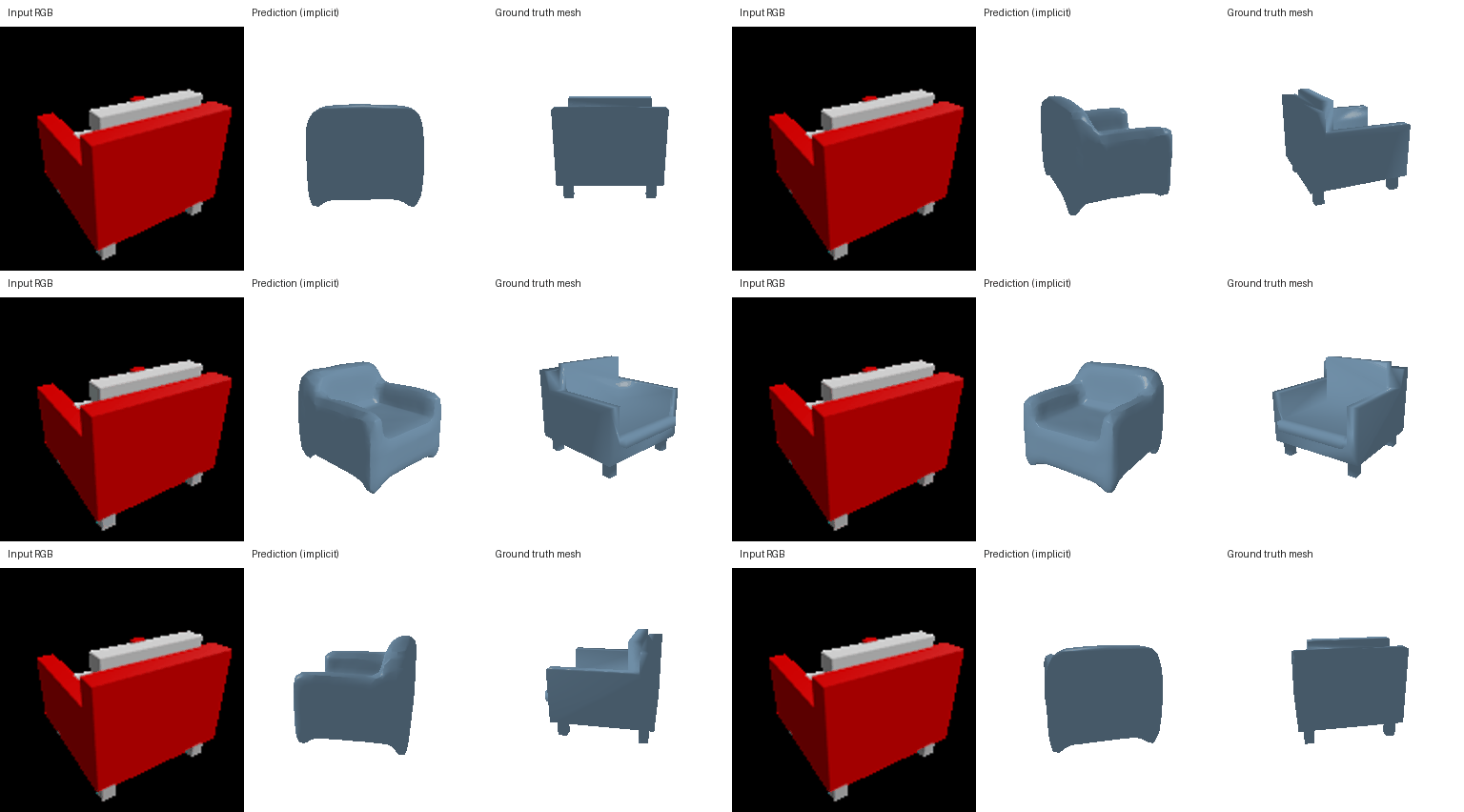
c04660caf4670baed40fb6f8053555de, view 00. F1@0.05: 85.85%.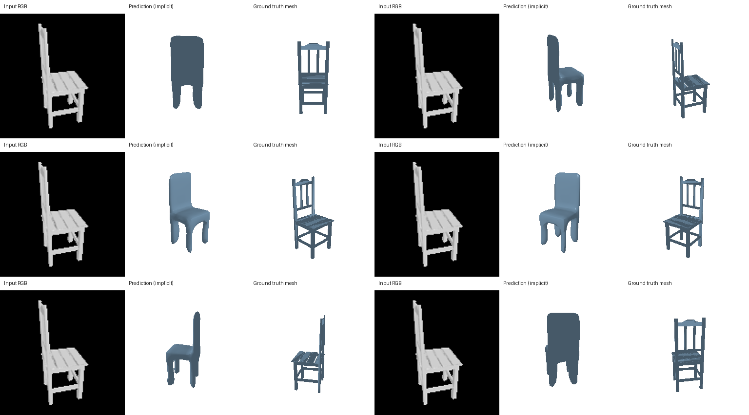
768ea32d8303095bfe6f9308e75765b1, view 00. F1@0.05: 90.99%.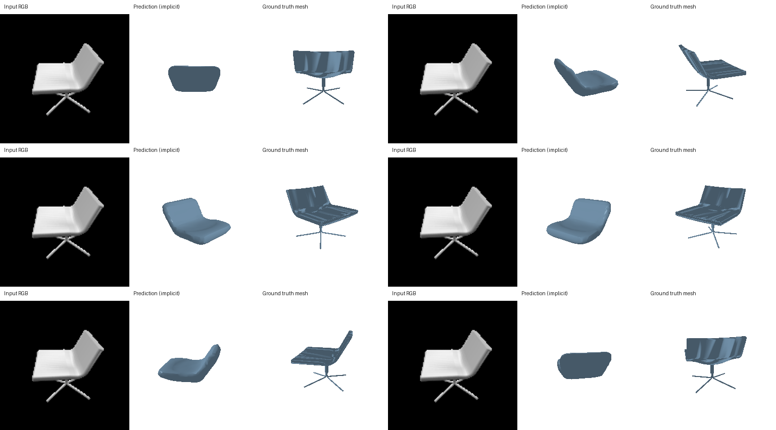
37235898ebd06b3b504721639e19f609, view 00. F1@0.05: 87.99%.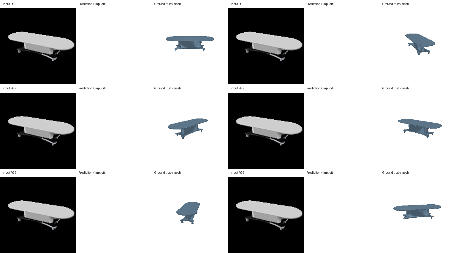
The implicit decoder changes test F1@0.05 by -3.91 percentage points relative to the convolutional voxel decoder. Both use the same occupancy targets and 32³ evaluation grid. The coordinate MLP shares a function across query locations; the convolutional decoder builds a spatial feature volume.
The first two examples recover a rounded seat/back outline, while the pedestal chair loses its narrow base. The lowest-scoring long bench has no extracted surface: its predicted occupancies do not cross the 0.5 threshold. The coordinate MLP also rounds away the thin slats visible in the targets.
Reproduction and checks
Fitting, training, evaluation, and rendering ran on NVIDIA GeForce RTX 5090 using PyTorch 2.8.0+cu128, CUDA 12.8, and PyTorch3D 0.7.9. The actual RGB point model reduced the two-chair smoke-test loss from 0.01041 to 0.00022 in 300 updates.
Tests check analytic BCE gradients, Chamfer values and gradients against a dense distance matrix, smoothing gradients, decoder dimensions, variable mesh batch sizes, empty surfaces, reproducible metrics, and checkpoint continuation against uninterrupted training.
python prepare_data.py
python fit_data.py --type vox
python train_model.py --type vox
python eval_model.py --type vox --load_checkpoint
python interpret.py --type point --run_dir runs/point
python build_report.py
python -m pytest -q tests
Setup and complete commands · Environment · Object splits · Results
Starter code and dataset: learning3d/assignment2, commit 7bb80cba23f59b87a01f489fcf373e74cd97fedb. Rendering and nearest-neighbor operations use PyTorch3D. The supplied evaluation conventions are retained.