1.3 Ray Sampling
1.4 Point Sampling
1.5 Volume Rendering

2. Optimizing a Basic Implicit Volume
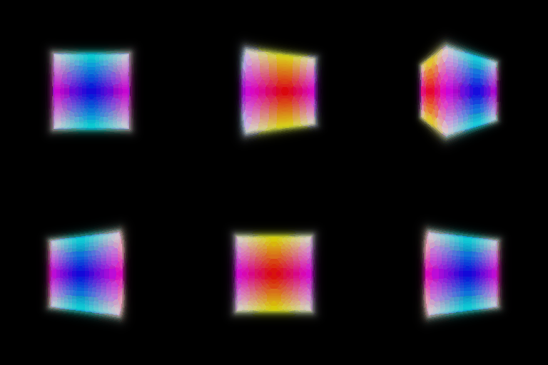
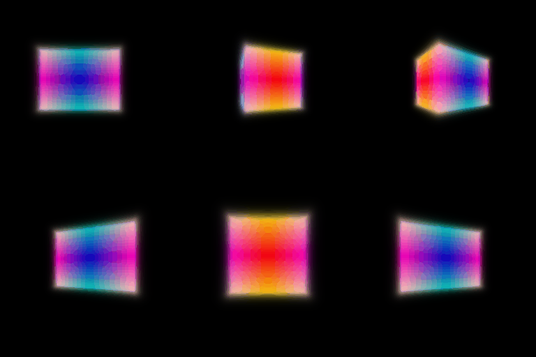
Optimized box center: (0.25, 0.25, 0.00). Side lengths: (2.01, 1.50, 1.50).
The optimized box is visually similar to the reference in its shape, proportions, and colors.
3. Optimizing a Neural Radiance Field

4.1 View Dependence
Without view dependence
With view dependence

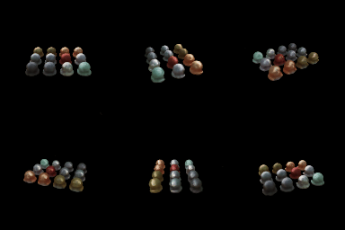
Both models were trained on Materials for 250 epochs at 128 × 128 resolution. Adding viewing direction lets the model represent changes in highlights and color, as seen on some objects in these renderings. However, greater view dependence also increases the risk of overfitting the training views, which can reduce rendering quality from new viewpoints.
4.3 VolSDF
Color
Geometry

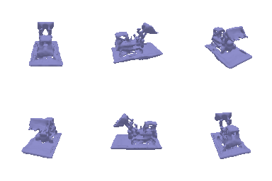
α and β: α scales volume density and therefore controls opacity. β controls the width of the transition from low density outside the surface to high density inside it.
- A high β makes density change more gradually across the surface, which can blur fine geometric details. A low β creates a sharper surface boundary, but requires more precise sampling.
- A higher β is generally easier to optimize because points farther from the surface can still provide useful gradients. A very low β creates a narrow density transition that may be missed by the ray samples.
- A lower β can give a more accurately located surface if training converges and sampling is sufficient. If β is too small, optimization can become difficult and some parts of the surface may be missed.
I used density α = 10, β = 0.05, 128 samples per ray, learning rate 0.0005, and 250 epochs at 128 × 128 resolution. The SDF network used geometric initialization with radius 1.0, Softplus with parameter 100, and Eikonal weight 0.1. Geometric initialization gives the SDF a simple spherical starting shape. The stronger Eikonal regularization encourages the SDF gradient magnitude to stay close to one, helping the network learn a valid signed distance function. Together, these settings reduced the large false surfaces observed in the baseline.
5.5 Gaussian Splatting

6.2 Training 3D Gaussian Representations
| Parameter | Learning rate |
|---|---|
| Means | 0.0001 |
| Scales | 0.005 |
| Colors | 0.01 |
| Opacities | 0.01 |
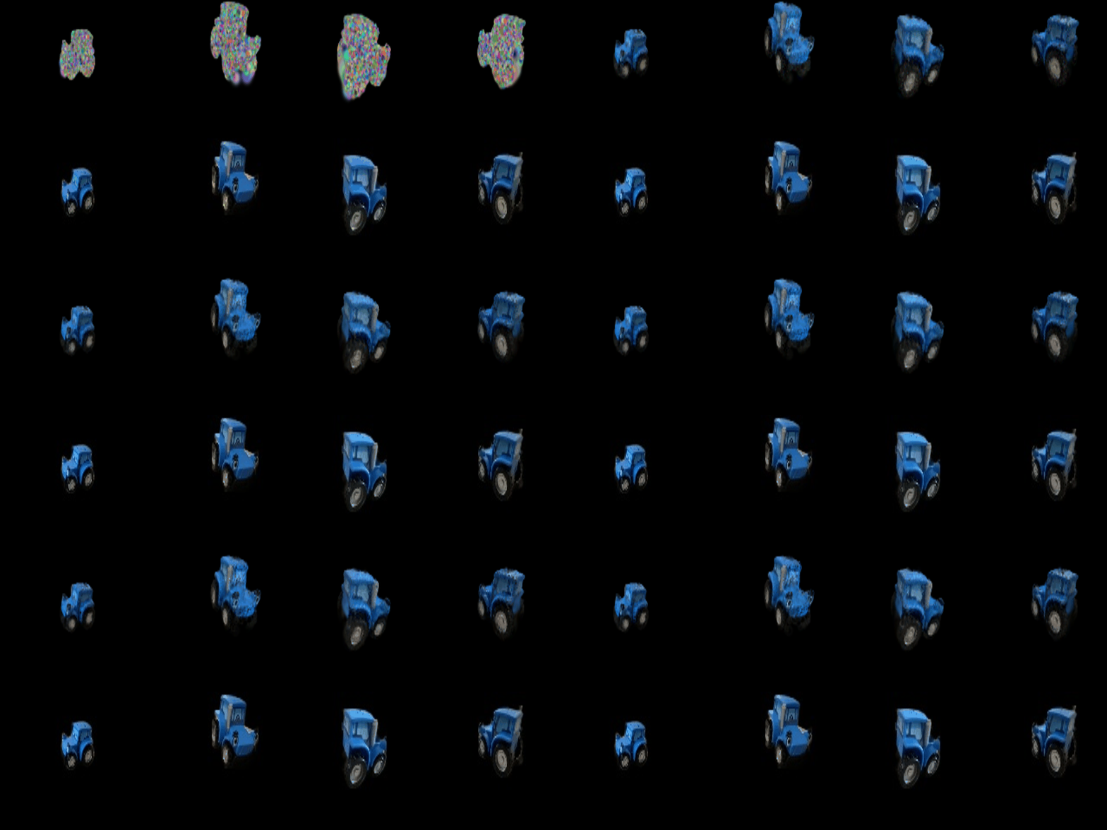
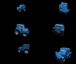
Training iterations: 1,000. Held-out mean PSNR: 28.612 dB. Held-out mean SSIM: 0.932.
7.1 Rendering Using Spherical Harmonics
DC only
Spherical harmonics

Frame 0


The green areas of the chair are darker with SH, and the gold pattern has stronger contrast. The DC version looks brighter and more uniform across the chair back. The chair shape is unchanged.
Frame 8
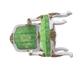

In this side view, SH changes the brightness of the green areas and metal frame, making the gold pattern more visible. DC assigns each Gaussian a fixed color, so it cannot model these changes with viewing direction.
Frame 24


The large beige area under the chair looks similar in both versions, while SH changes the shading along the edges and legs. The difference is smaller than in the front view.