1. Differentiable Volume Rendering
1.3 Ray sampling
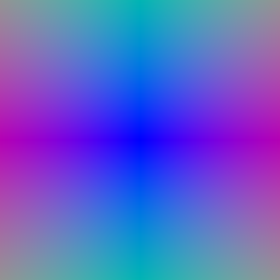
I generated a 2D pixel grid in [−1, 1], following the PyTorch3D image-axis convention. Pixel coordinates with a depth of 1 were unprojected into world space. Each ray starts at the camera center, and its direction is the normalized vector toward the unprojected point.

1.4 Point sampling
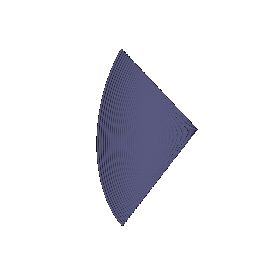
For each ray, I uniformly sampled 64 distances between 0 and 5 and computed points using p(t) = o + td. Both the sample positions and distances are stored in the RayBundle.
1.5 Color and depth aggregation
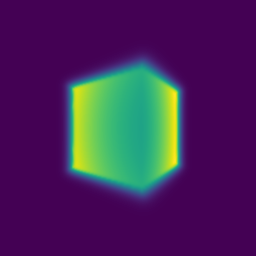
I implemented emission–absorption rendering with αᵢ = 1 − exp(−σᵢΔtᵢ), Tᵢ = exp(−Σⱼ<ᵢ σⱼΔtⱼ), and wᵢ = Tᵢαᵢ. The first sample has transmittance 1. RGB is Σᵢ wᵢcᵢ, and depth is Σᵢ wᵢtᵢ.

2. Optimizing a Basic Implicit Volume
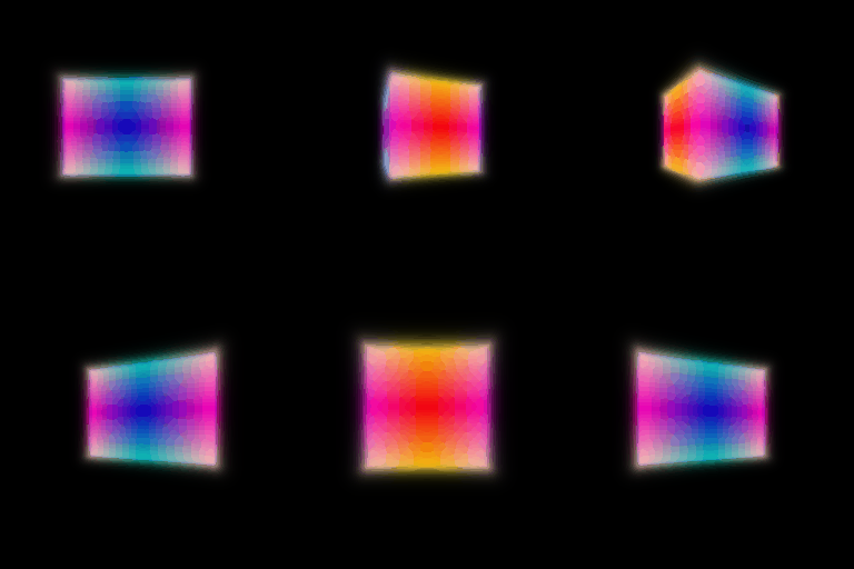
I randomly selected 4,096 pixels per image and minimized the RGB mean squared error between the rendered box and four provided target images with known camera poses. Adam optimized the box center and three side lengths; the renderer remained the same as in Part 1.
The supplied training configuration uses 1,000 epochs, an initial learning rate of 0.0005, and 256 × 256 images.


| Required parameter | Final value, rounded to two decimals |
|---|---|
| Box center | (0.25, 0.25, 0.00) |
| Box side lengths | (2.01, 1.50, 1.50) |
3. Optimizing a Neural Radiance Field
I represented the Lego scene with a position-dependent MLP. Six positional-encoding frequencies plus the original xyz coordinates produce 39 input features. The backbone has six linear layers, 128-dimensional hidden features, and an input skip at layer index 3. Separate linear heads output density through ReLU and RGB through Sigmoid. Viewing direction is not used in this part.
| Images / resolution | 100 training views / 128 × 128 |
|---|---|
| Training | 250 epochs; Adam; RGB MSE |
| Initial learning rate | 0.0005, multiplied by 0.8e/50 after e scheduler steps |
| Sampling | 1,024 rays per update; 128 points per ray; near/far = 2/6 |

The yellow body, bucket, tracks, and base are recognizable and remain broadly consistent across views. Small components and edges are still blurred, with a faint artifact below the base. The final displayed batch MSE at epoch 249 was 0.004146. This is a single training batch value, not an epoch average or a held-out metric. The originally saved GIF was produced at epoch 240 under the earlier periodic rendering schedule.
4.1 View Dependence
I added direction information only to the color branch, keeping density dependent on position. The normalized camera-to-sample ray direction is encoded with two frequencies, producing 15 features. These are concatenated with the 128 position features and passed through a 143 → 64 → 3 color MLP with ReLU and a final Sigmoid.
The materials configuration uses 128 × 128 images, 1,024 rays per update, 128 samples per ray over distances 1–7, and Adam with an initial learning rate of 0.0001. The recorded checkpoint reached epoch 250; the configured range is epochs 0–250.

Multiple objects and their different colors can be distinguished, although material details and boundaries remain soft. Direction dependence allows the model to express highlights that cannot be represented by a fixed color at each position. However, a high-capacity direction branch can also memorize training views or compensate for incorrect geometry, reducing consistency at unseen viewpoints.
Using only two directional frequencies and introducing direction late in the network limits this capacity while retaining view-dependent appearance. This is a design trade-off, not proof that overfitting is eliminated. No matched materials experiment without direction input was recorded, so I do not claim a measured improvement over a position-only baseline.
4.2 Coarse/Fine Sampling
I trained two independent position-only NeRF networks. The coarse pass evaluates 64 uniformly spaced points. Its detached rendering weights define a piecewise-constant PDF between sample midpoints. Inverse-CDF sampling selects 64 additional distances; the fine network evaluates the sorted union of the original and new samples, totaling 128 points. I add a small positive weight before normalization to handle empty rays. Evaluation uses deterministic quantiles.
Both networks receive RGB supervision: L = MSE(Cfine, Cgt) + MSE(Ccoarse, Cgt). The fine network produces the displayed RGB and depth. Training used 250 epochs, 128 × 128 images, 1,024 rays per update, and Adam with an initial learning rate of 0.0005.

Speed and quality trade-off
The hierarchical result preserves the main Lego structure, with recognizable bucket, tracks, and body. Differences in fine details are subtle at 128 × 128, and some edge artifacts remain. The method spends more fine samples near regions that contributed to the coarse rendering instead of distributing all samples uniformly.
| Method | Networks | Point queries per ray |
|---|---|---|
| Part 3 | 1 | 128 |
| Part 4.2 | 2 | 64 coarse + 128 fine = 192 |
This configuration increases point queries by 50%, introduces a second network, and adds PDF construction and sampling overhead. It is therefore not an equal-compute comparison, and hierarchical sampling is not automatically faster. In the recorded PSC run, the median completed-epoch training-loop throughput was 39.84 updates/s over 250 epochs; periodic rendering is excluded. A same-hardware timing of the Part 3 baseline was not recorded, so a measured speedup cannot be reported.
The last displayed batch loss was 0.007766, summing coarse and fine MSE. It is not directly comparable to the single-network loss in Part 3.
4.3 VolSDF
I implemented a neural signed distance field with negative values inside the object and positive values outside. Its zero level set defines the surface. The distance network uses six linear layers with 128-dimensional hidden features and six positional-encoding frequencies. It predicts a residual added to a radius-1 sphere SDF; zero-initializing the final residual layer starts training from a sphere. A separate two-layer color MLP predicts RGB through Sigmoid.
The density conversion is the scaled Laplace CDF applied to the negative SDF:
σ(s) = α × 0.5 exp(−s/β) for s ≥ 0, and σ(s) = α × [1 − 0.5 exp(s/β)] for s < 0.
The objective combines RGB MSE with 0.02 × mean((‖∇s‖₂ − 1)²). The Eikonal term encourages distance-like spatial gradients. I compared β = 0.10, 0.05, and 0.02 while keeping α = 10 and the other configured settings unchanged: 250 epochs, 128 × 128 images, 1,024 rays per update, 128 samples per ray over distances 2–6, and an initial Adam learning rate of 0.0005. The color and geometry branches do not use viewing direction.
Selected result: β = 0.02

I selected β = 0.02 for the clearest overall RGB rendering and the more localized base and vehicle structure among these three runs. The recovered surface still has irregular edges and imperfect small components, and its geometry is not evaluated against a ground-truth mesh. A nonempty extracted mesh establishes recovery of a zero level set, not exact surface accuracy.
Parameters and required questions
- What do α and β do? α scales the density and therefore absorption. β sets the width of the smooth transition around the zero level set. At the surface the density is α/2; inside, it approaches α, and outside it decays toward zero.
- How do high and low β bias the learned SDF? A high β spreads density across a wider neighborhood of the surface, allowing a more diffuse rendering and weaker localization of the boundary. A low β makes density more tightly coupled to the surface. The exact geometric displacement also depends on α, sampling, and image supervision; it is not necessarily a uniform expansion or contraction.
- Which is easier to train? A larger β is generally easier early in training because useful image gradients extend farther from the current surface. With a very small β, coarse ray samples can miss the narrow transition and provide weaker optimization signals.
- Which can give a more accurate surface? A smaller β can better localize the boundary if the optimization converges and ray sampling is sufficiently dense. If β is too small for the sampling budget, training can instead become unstable or inaccurate.
Hyperparameter comparison
All three runs completed 250 epochs and produced color and geometry renderings. Each GIF contains 20 views at 128 × 128. The table reports the final training batch objective, which includes the Eikonal term; it is neither an epoch average nor a held-out metric.
| β (α = 10) | Color | Geometry | Final batch loss | Observation |
|---|---|---|---|---|
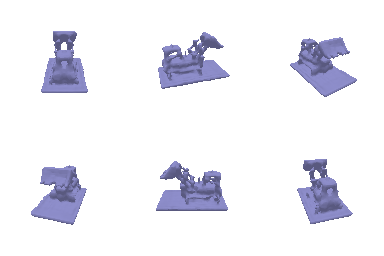
| 0.10 |  |  | 0.009025 | Soft RGB boundaries and the broadest, most rounded base. Small vehicle structures appear smoothed together. |
| 0.05 |  | 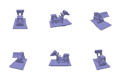 | 0.007572 | Lowest final batch objective; a more localized base than 0.10, but visible colored haze and speckles around the object in some views. |
| 0.02, selected | | | 0.007649 | Cleaner surrounding background and more distinct RGB details in the inspected views. Geometry retains smaller structures, with some roughness remaining. |
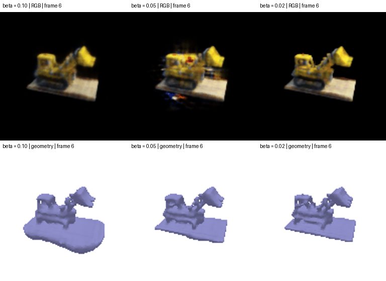
A smaller β narrows the density transition, which is consistent with the sharper localization seen here. The sphere initialization supplies a surface from the start, and the Eikonal term encourages distance-like gradients. The β = 0.02 run trains successfully at the current sampling budget, although this does not imply that reducing β further would improve it.
β = 0.05 has a slightly lower final batch loss than β = 0.02, but the latter is preferable in the inspected renderings. A single image-space training loss does not rank geometric quality. These are one run per setting, without a controlled common random seed, so the comparison supports a qualitative choice among the available runs rather than a statistically established optimum.
5. 3D Gaussian Rasterization
I implemented 3D covariance construction from rotation and scale, projection to 2D means and covariances, and evaluation of the 2D Gaussian power. Gaussians behind the camera are removed and the remainder are sorted from near to far. Alpha and transmittance are then accumulated to produce RGB, depth, and a silhouette mask. The implementation passed all four supplied Gaussian unit tests.
The scene contains 283,873 pretrained chair Gaussians. Rendering uses 32 camera views at 256 × 256, with minibatch splatting to control memory. No scene training is performed in this part.

6. Training 3D Gaussian Representations
I initialized 10,000 isotropic Gaussians from the provided truck point cloud and optimized their means, log-scales, colors, and opacity logits. Rotations are not optimized for isotropic Gaussians. Each update renders one training view with a black background and minimizes standard L1 image loss.
| Parameter / setting | Value |
|---|---|
| Mean learning rate | 0.0001 |
| Log-scale learning rate | 0.005 |
| Color learning rate | 0.01 |
| Opacity-logit learning rate | 0.01 |
| Optimizer / iterations | Adam / 1,000 |
| Training resolution | 160 × 90 |
| Held-out mean PSNR | 28.737 dB |
| Held-out mean SSIM | 0.934 |
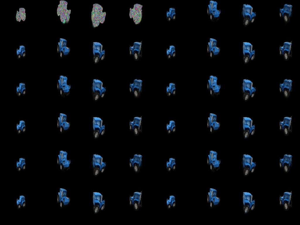
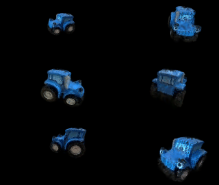
The trained representation recovers the blue body, wheels, and overall truck silhouette. Small details remain soft. The held-out evaluation reports a mean PSNR of 28.737 dB and a mean SSIM of 0.934, indicating substantial agreement with the reference images while leaving reconstruction error.
7.1 Rendering Using Spherical Harmonics
I loaded the pretrained chair's degree-0 through degree-3 real spherical harmonic coefficients: 16 coefficients for each RGB channel. For each Gaussian, I normalize the camera-to-Gaussian direction, evaluate the 16 basis functions, sum their RGB-weighted contributions, add 0.5, and clamp negative values to zero. Gaussian positions, scales, rotations, and opacities remain unchanged; no SH training is performed.

Same-view RGB comparisons


7.2 Training on a Harder Scene
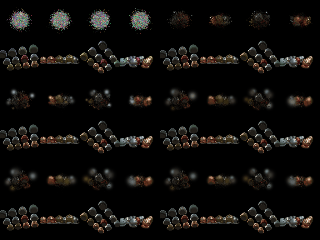
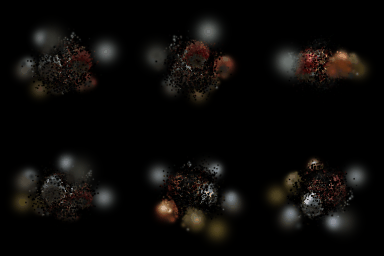
I trained 10,000 isotropic Gaussians on materials from random initialization. The baseline reuses the truck's optimizer rates and L1 loss, with init_type="random". Both experiments use seed 0, 1,000 updates, 128 × 128 images, and 512 Gaussians per splat. The initial scene is random in both cases; no ground-truth point cloud is used.
Changes in the improved configuration
- Multiply the initial random means by 4, expanding coordinate standard deviation from 0.2 to 0.8 to cover more of the multi-object scene.
- Set initial isotropic scales to 0.03 instead of the original random values below approximately 0.01.
- Set initial opacity to 0.1 instead of sigmoid(8), reducing initial occlusion.
- Increase the mean learning rate to 0.002 and exponentially decay it to 0.0002 over training. Other parameter rates and the L1 loss are unchanged.
| Setting / result | Baseline | Improved |
|---|---|---|
| Mean learning rate | 0.0001 | 0.002 → 0.0002 |
| Log-scale / color / opacity-logit LR | 0.005 / 0.01 / 0.01 | 0.005 / 0.01 / 0.01 |
| Iterations | 1,000 | 1,000 |
| Mean PSNR (dB) | 17.487 | 22.576 |
| Mean SSIM | 0.624 | 0.816 |
| Final displayed training L1 | 0.088 | 0.039 |
Evaluation uses the same 100-view validation split in both runs, following the supplied script; these are not test-split metrics. The improved run gains 5.089 dB PSNR and 0.192 SSIM. Each result is from one seed. Because several settings changed together, the experiment establishes the combined effect, not the individual contribution of each change.
Baseline
Improved
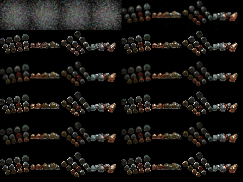
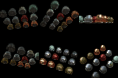
The baseline leaves much of the scene fragmented, with diffuse blobs and missing surfaces. The improved configuration recovers distinct objects and substantially more of their arrangement and appearance, although edges and fine material details remain imperfect. Broader initial coverage and larger initial scales help place useful support across the scene; lower opacity reduces premature occlusion, while faster early position updates allow larger corrections. These are plausible explanations consistent with the result, rather than conclusions from isolated ablations.