The geometry is directly optimized in these experiments. The animations compare the optimized representation with the ground truth.
1.1 Fitting a voxel grid1.2 Fitting a point cloud1.3 Fitting a mesh
Voxel: Binary cross-entropy with logits supervises occupancy.
Point cloud: A custom symmetric squared Chamfer loss matches the two point sets.
Mesh: Sampled-surface Chamfer loss is combined with uniform Laplacian regularization to encourage smooth geometry.
2. Reconstructing 3D from a Single View
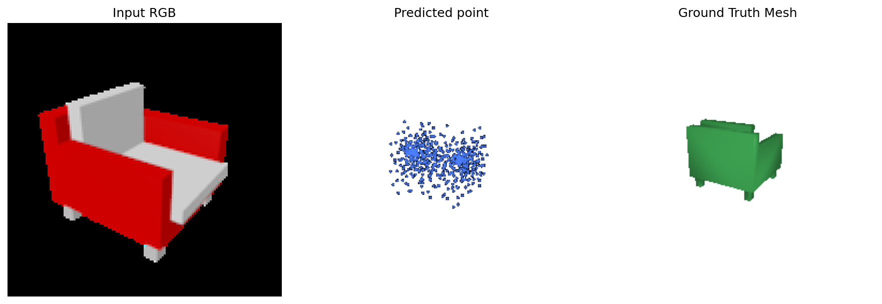
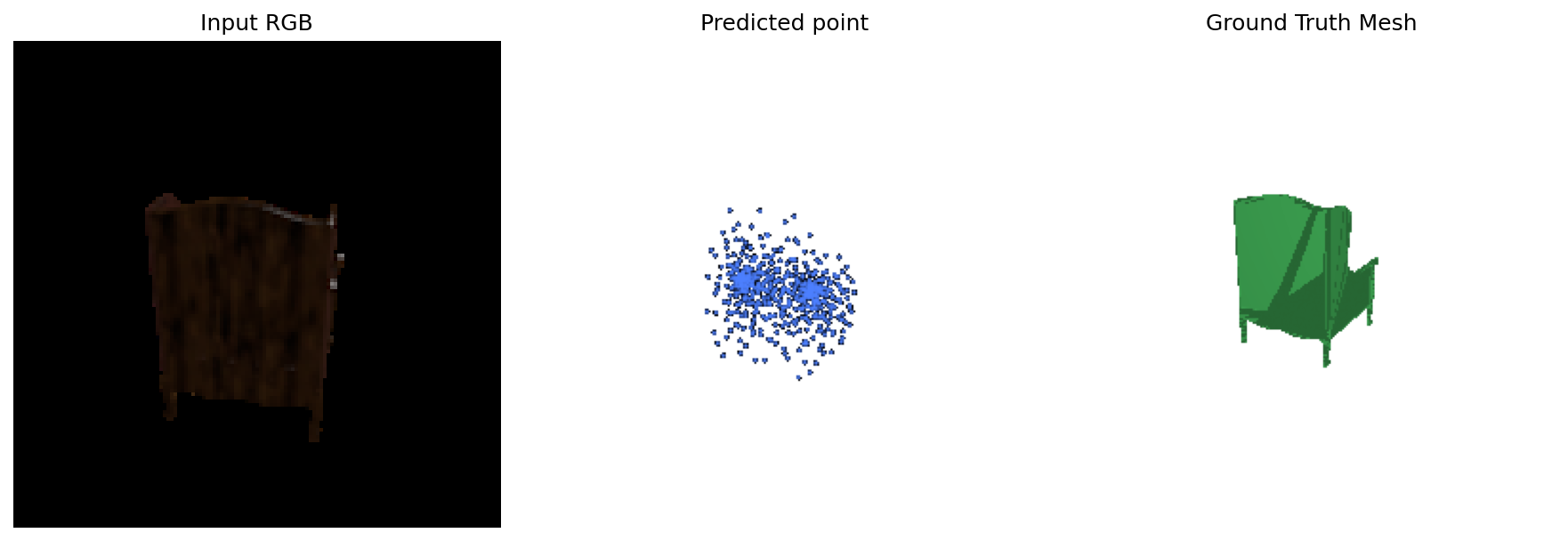
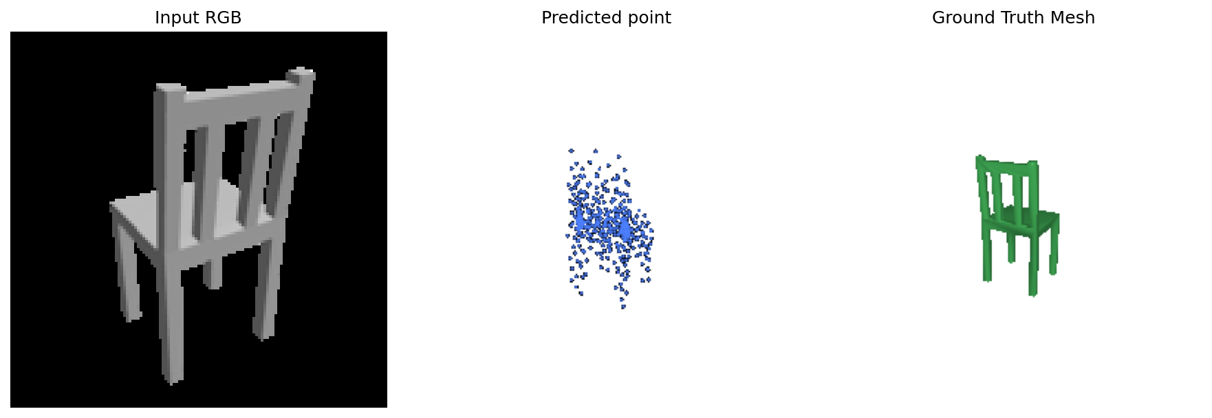
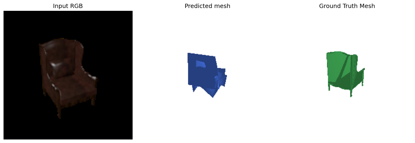
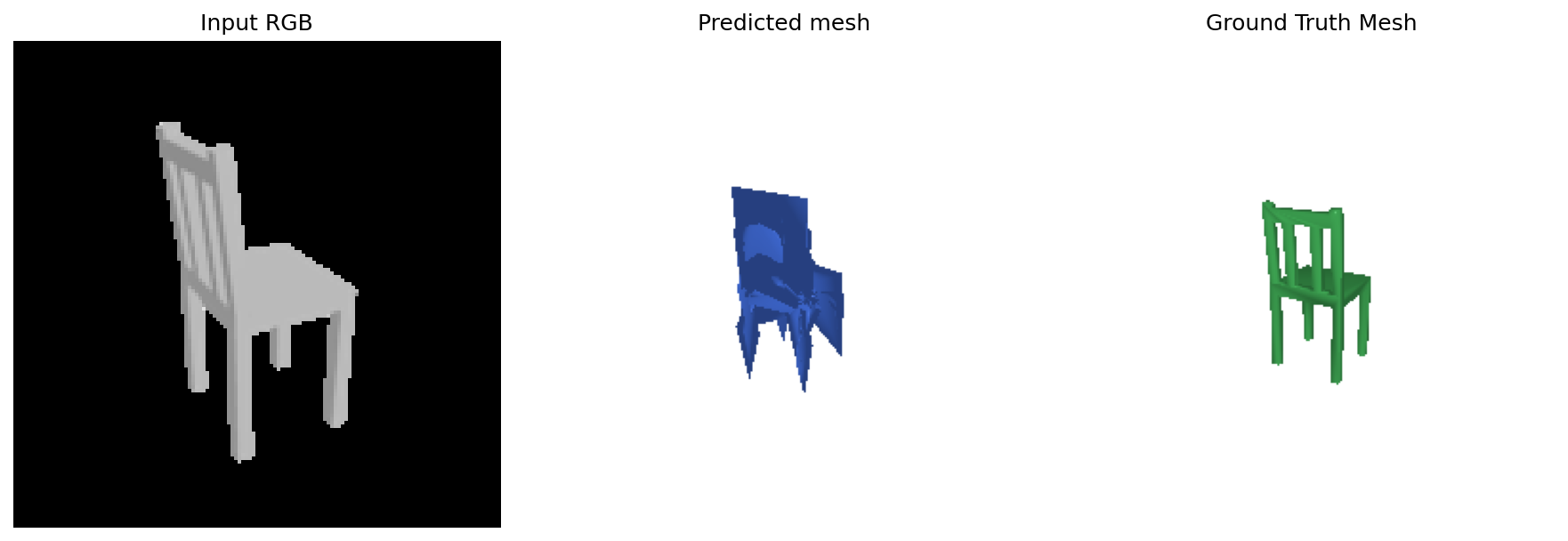
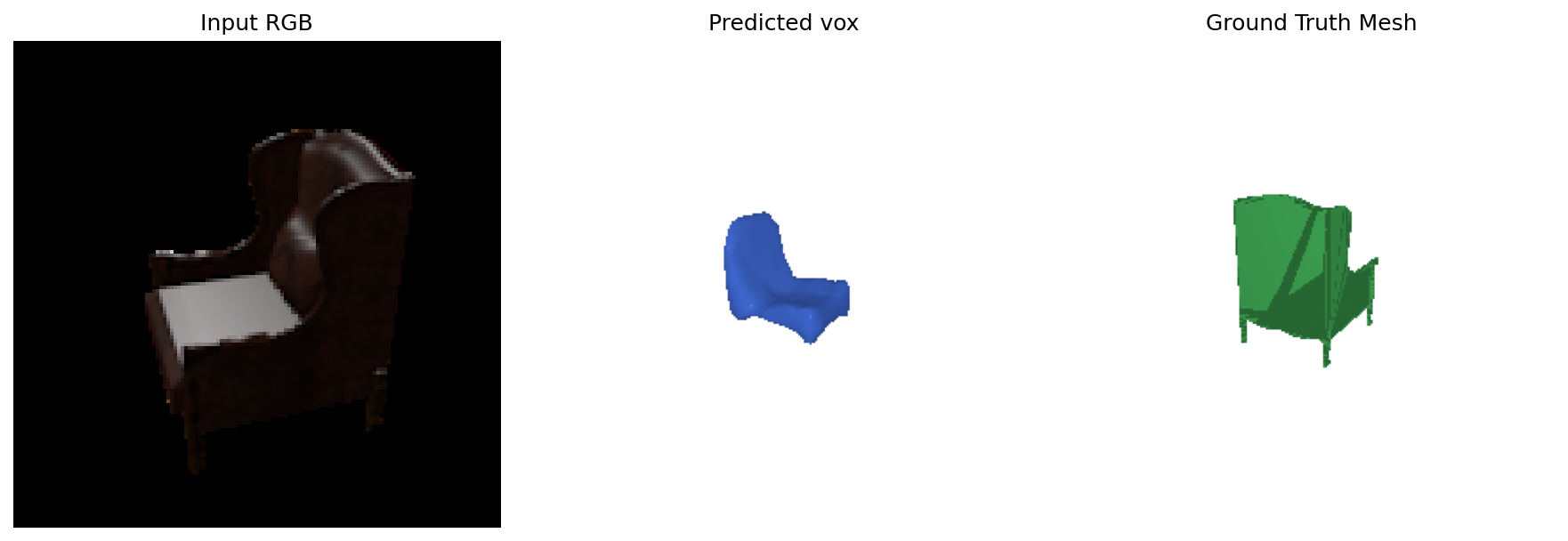
A ResNet18 encoder produces a 512-dimensional image feature. Each decoder maps this feature to a different 3D representation. Each image below shows the input RGB, predicted geometry, and ground-truth mesh, from left to right.
2.1 Image to Voxel Grid
A fully connected layer followed by 3D transposed convolutions predicts a 32 × 32 × 32 occupancy grid. Marching cubes extracts the surface at occupancy 0.5.
Test example 000Test example 002Test example 005
2.2 Image to Point Cloud
An MLP with dimensions 512 → 1024 → 2048 → 3000 predicts 1,000 unordered 3D points, trained with Chamfer loss.
Test example 000Test example 002Test example 005
2.3 Image to Mesh
An MLP predicts offsets for the 2,562 vertices of a level-4 ico-sphere. The loss combines sampled-surface Chamfer distance and Laplacian smoothing.
Test example 000Test example 002Test example 005
Quantitative Comparison
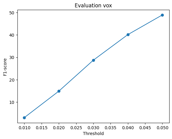
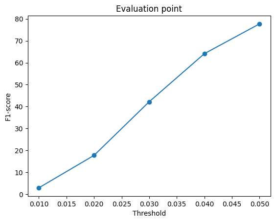
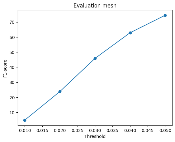
VoxelPoint cloudMesh
Representation
Avg F1@0.05 (/100)
Voxel grid
47.580
Point cloud
77.834
Mesh
74.490
The reported validation averages show point cloud > mesh > voxel at threshold 0.05. Point clouds can represent geometry without the fixed connectivity of a mesh template, while connected mesh surfaces provide a continuity prior. A 32³ voxel grid can lose thin structures such as chair legs. Mesh predictions may still contain folds, and a higher F1 at a relaxed distance threshold does not guarantee better topology or fine detail.
2.4 Effect of Learning Rate
The voxel model is compared using learning rates of 1e-4, 4e-4, and 1e-3. All three available experiment checkpoints record step 6000. The same test indices, 000, 002, and 005, are shown below.
Among the three tested learning rates, 4e-4 achieves the highest average F1@0.05 (47.580), followed by 1e-4 (39.953) and 1e-3 (30.298). The 4e-4 run exceeds 1e-4 by 7.627 F1 points and 1e-3 by 17.282 points under the same specified training iteration budget. Thus, 4e-4 is the best-performing setting in these reported runs, not necessarily the optimal learning rate for every training configuration.
In example 005, the 1e-3 result contains small disconnected fragments, while lower learning rates retain part of the chair back. This qualitative observation is consistent with the lower average F1 of the 1e-3 run. A larger learning rate may make updates less stable, while 1e-4 may need more iterations to converge. The intermediate rate may offer a better balance between progress and stability within this training budget. These are hypotheses: F1 alone does not establish the optimization dynamics or prove underfitting or instability.
2.5 Model Interpretation: Input Occlusion
For each test image, the upper, middle, or lower third of the foreground bounding box is filled with black. The same voxel checkpoint predicts geometry from the original and masked images without retraining. F1@0.05 uses 1,000 surface samples, with fixed GT samples shared across all four variants of each example and metric seed 0.
Test Example
Input
F1@0.05 (/100)
Drop from Original
000
Original
87.135
+0.000
000
Upper
54.648
+32.487
000
Middle
85.792
+1.342
000
Lower
59.836
+27.298
002
Original
68.980
+0.000
002
Upper
67.322
+1.659
002
Middle
49.166
+19.814
002
Lower
82.386
-13.406
005
Original
30.515
+0.000
005
Upper
31.014
-0.499
005
Middle
65.043
-34.528
005
Lower
5.258
+25.257
Drop = original F1 minus masked-input F1, in F1 points. Positive values indicate degradation; negative values indicate improvement. Values are computed before rounding, so displayed differences may differ by 0.001 when calculated from the rounded F1 values.
Test example 000: original and three occlusion conditionsTest example 002: original and three occlusion conditionsTest example 005: original and three occlusion conditions
Example 000: Upper and lower occlusion substantially reduce F1 by 32.487 and 27.298 points, while middle occlusion changes it by only 1.342 points. For this input, the prediction is more sensitive to information in the upper and lower image bands.
Example 002: Middle occlusion produces the largest drop (19.814 points), whereas lower occlusion improves F1 from 68.980 to 82.386.
Example 005: Lower occlusion reduces F1 from 30.515 to 5.258, while middle occlusion improves it to 65.043. Thus, removing image information does not uniformly reduce the measured reconstruction quality. Suppression of misleading image cues is one possible explanation, but these three examples do not establish the cause or demonstrate a general benefit from occlusion.
Under lower occlusion, example 005 retains only 3 occupied voxels, with precision 100.0 but recall only 2.7. The low F1 shows that a small matching fragment can have high precision yet miss almost the entire target surface. Its mean absolute probability change is only about 0.017, illustrating that small probability changes near occupancy 0.5 can substantially alter the extracted surface.
3.1 Implicit Occupancy Network
The implicit decoder predicts occupancy as a function of an image feature and a 3D query coordinate: f(image feature, x, y, z).
A 32 × 32 × 32 meshgrid is generated in [-1, 1]³. Each coordinate is concatenated with the 512-dimensional feature and passed through an MLP: 515 → 256 → 256 → 128 → 1. The 32,768 queries are processed in chunks of 2048. Outputs are occupancy logits, trained with binary cross-entropy; sigmoid converts them to probabilities for evaluation.
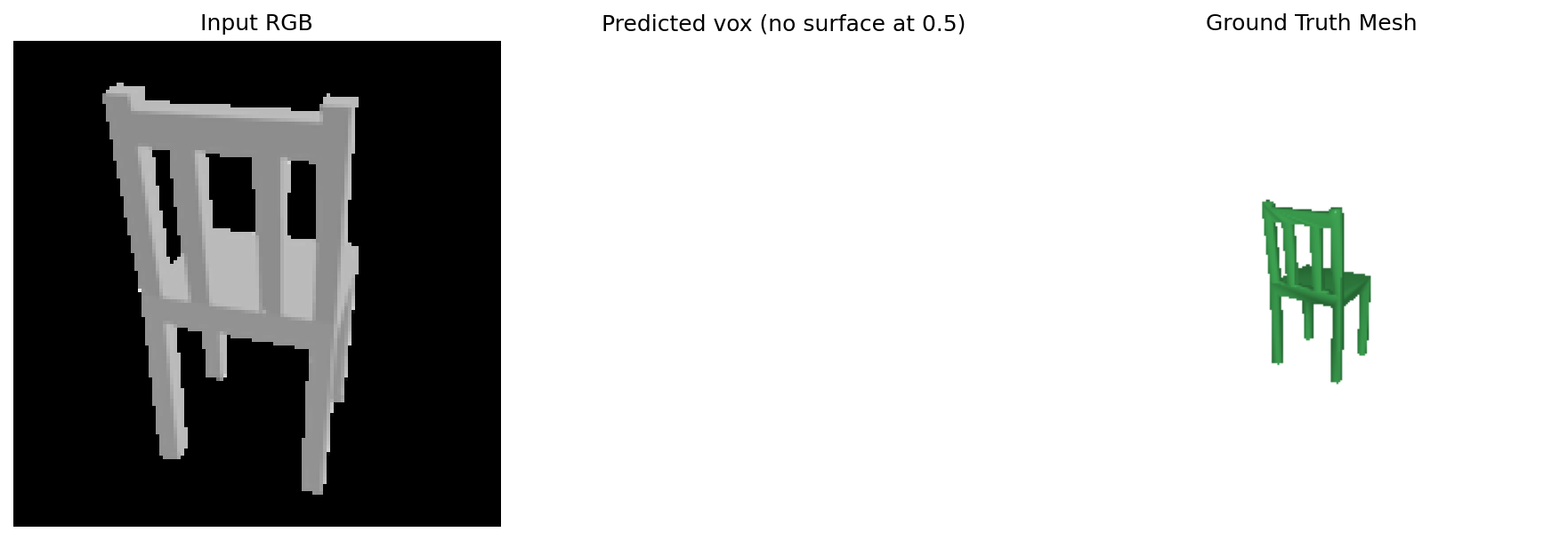
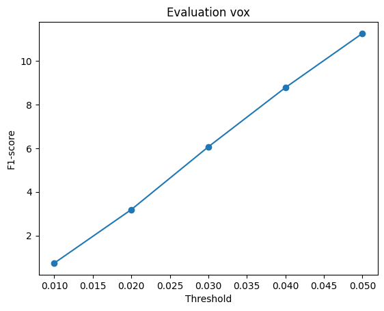
Implicit network: test example 000Implicit network: test example 002Implicit network: test example 005Implicit evaluation curve; older output names still use “vox”.
The supplied curve gives an approximate F1@0.05 of 11.3, below the explicit voxel baseline. The fragmented predictions suggest several possible explanations. One possibility is a bias toward predicting empty space: if empty locations dominate the target grid, the unweighted binary cross-entropy loss may favor conservative occupancy predictions, allowing loss to decrease even when substantial parts of the chair are missed. If many occupancy probabilities remain below or near 0.5, surface extraction could retain only small fragments.
Another possibility is limited geometric learning in the simple MLP. Unlike the convolutional decoder, it has no explicit local convolutional structure, which may make it harder to learn coherent surfaces and thin chair parts from a global image feature. Training configuration may also contribute: the learning rate and iteration budget used for the voxel baseline may not suit this decoder, and the implicit model may require different settings or more training to converge. These are plausible hypotheses, not confirmed causes; checking occupancy distributions, training curves, and controlled decoder comparisons would help distinguish them.