
16-825 Learning for 3D Vision · Assignment 2
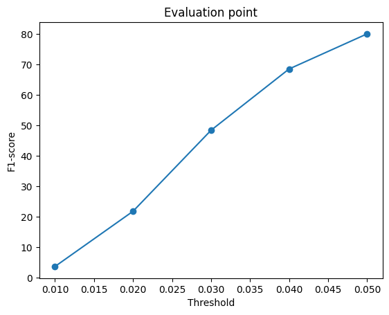
Chair reconstruction from one RGB image on R2N2 ShapeNet (single class, 678 test models). Every learned model uses a pretrained ResNet18 encoder, is trained end to end from images for 10k iterations (batch 32, Adam, lr 4e-4) and is scored by F1 at a 0.05 distance threshold on 1000 sampled points.
| Section | Representation | Decoder | F1@0.05 |
|---|---|---|---|
| 2.1 | Voxel grid 32³ | FC → 3D transposed conv | 54.9 |
| 2.2 | Point cloud (1000) | MLP → 1000×3 | 79.2 |
| 2.3 | Mesh (ico_sphere 4) | MLP → vertex offsets | 72.9 |
| 2.4 | Mesh, best w_smooth |
same as 2.3 | 75.3 (w=0) |
| 3.1 | Implicit occupancy | MLP(feature, xyz) on 32³ grid | 50.0 |
| 3.1 | Implicit occupancy (ONet) | conditional-BN ResNet on random points | 55.2 |
| 3.2 | Parametric (8 patches) | MLP(feature, uv, patch id) | 75.0 |
| 3.3 | Point cloud, trained on chair + car + plane | same as 2.2 | 79.8 on chairs (87.8 on all 3 classes) |
How to read the example gifs: each shows three turntables side by side. From left to right they are the input image, the ground-truth mesh and the prediction. The input image is fixed; the other two rotate 360°. Each is centered and scaled to fit the frame, so size differences between panels are not errors.
Each gif shows the optimized source on the left and the target on the right.


F1@0.05 = 54.9
The decoder maps the 512-d feature through a fully connected layer to a 128×4×4×4 volume. Three stride-2 3D transposed convolutions with BatchNorm and ReLU upsample it to 32³, and a final 3×3×3 convolution outputs one occupancy logit per voxel. Training uses BCE with logits; evaluation thresholds the sigmoid at 0.5 with marching cubes.
Examples (input · ground truth · prediction):


Predictions are smooth and blobby: they capture overall volume and pose but fill in the gaps between slats and legs. On 32 of 678 test chairs no voxel reaches 0.5, and those score 0. The loss weights every voxel equally and roughly 95% of the grid is empty, so for thin chairs the network prefers predicting empty.
F1@0.05 = 79.2
An MLP (512 → 1024 → 2048 → 1000×3, ReLU) regresses point coordinates directly and is trained with the chamfer loss from 1.2.
Examples (input · ground truth · prediction):
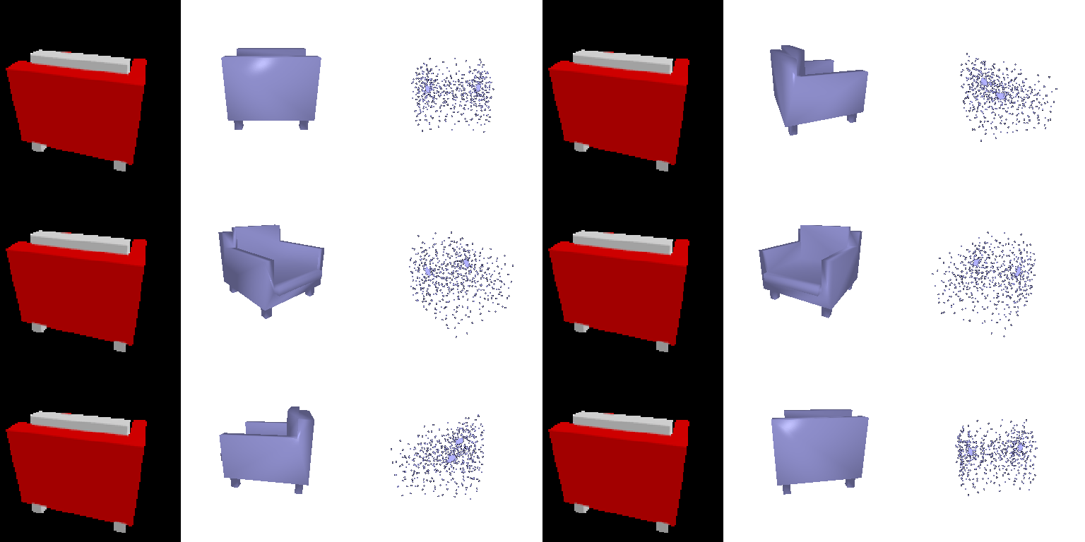
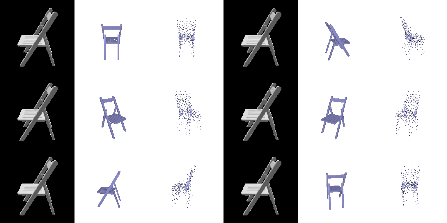
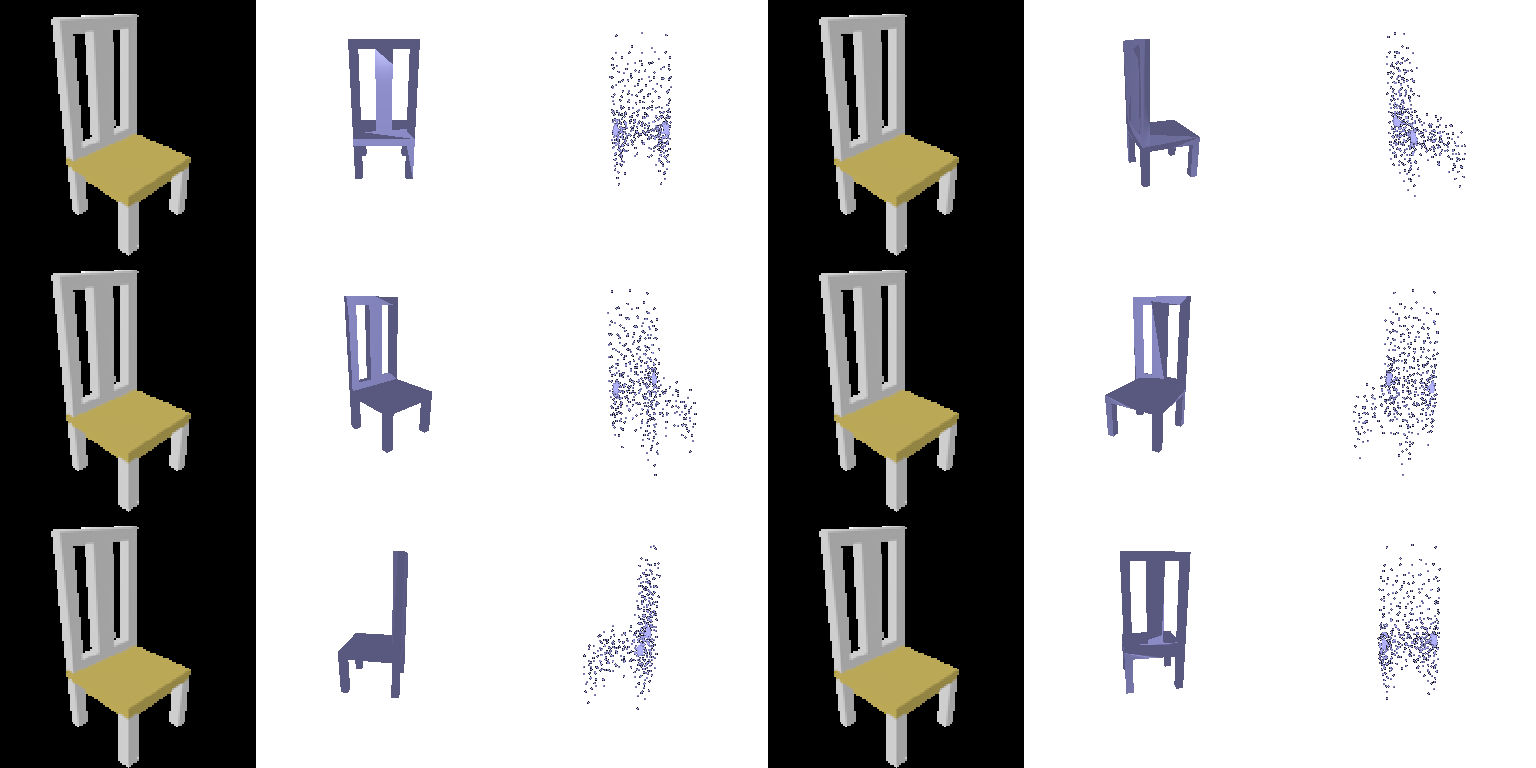
F1@0.05 = 72.9
The same MLP shape outputs a 3D offset for each of the 2562 vertices of a level-4 ico_sphere. The loss is chamfer on 1000 surface samples plus 0.1 × uniform Laplacian smoothing.
Examples (input · ground truth · prediction):
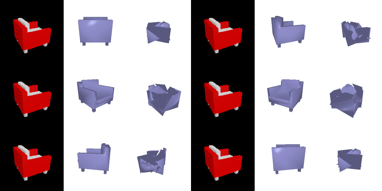


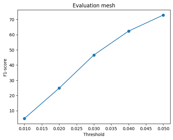
Comparison: point 79.2 > mesh 72.9 > voxel 54.9.
I varied w_smooth, the weight on the Laplacian term in
the mesh loss, and kept everything else fixed (ico_sphere level 4, 1000
samples, 10k iterations). The 2.3 baseline used 0.1.
w_smooth |
0 | 0.01 | 0.1 | 1 | 10 |
|---|---|---|---|---|---|
| F1@0.05 | 75.3 | 74.8 | 72.9 | 70.4 | 56.6 |
The same three test chairs are shown for each setting, all at the same turntable angle.


w_smooth=10. Chamfer is
the only term that F1 measures, so any weight moved to the Laplacian
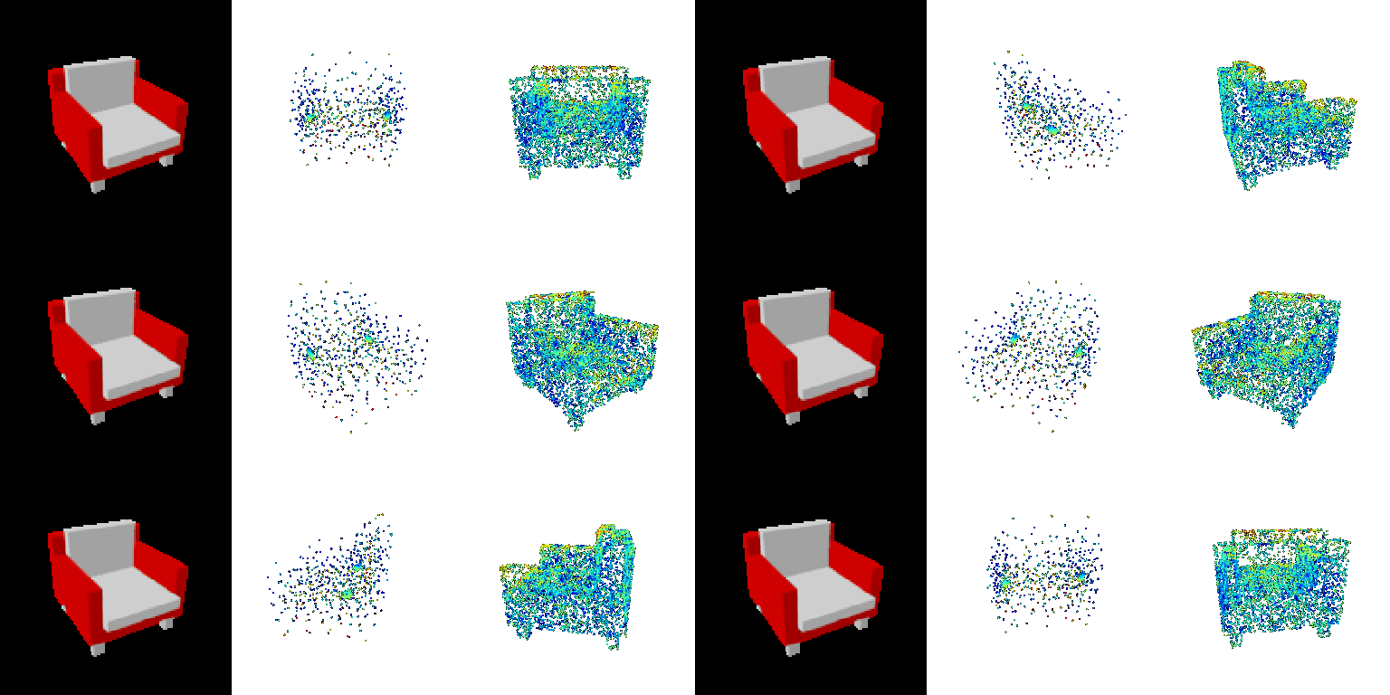
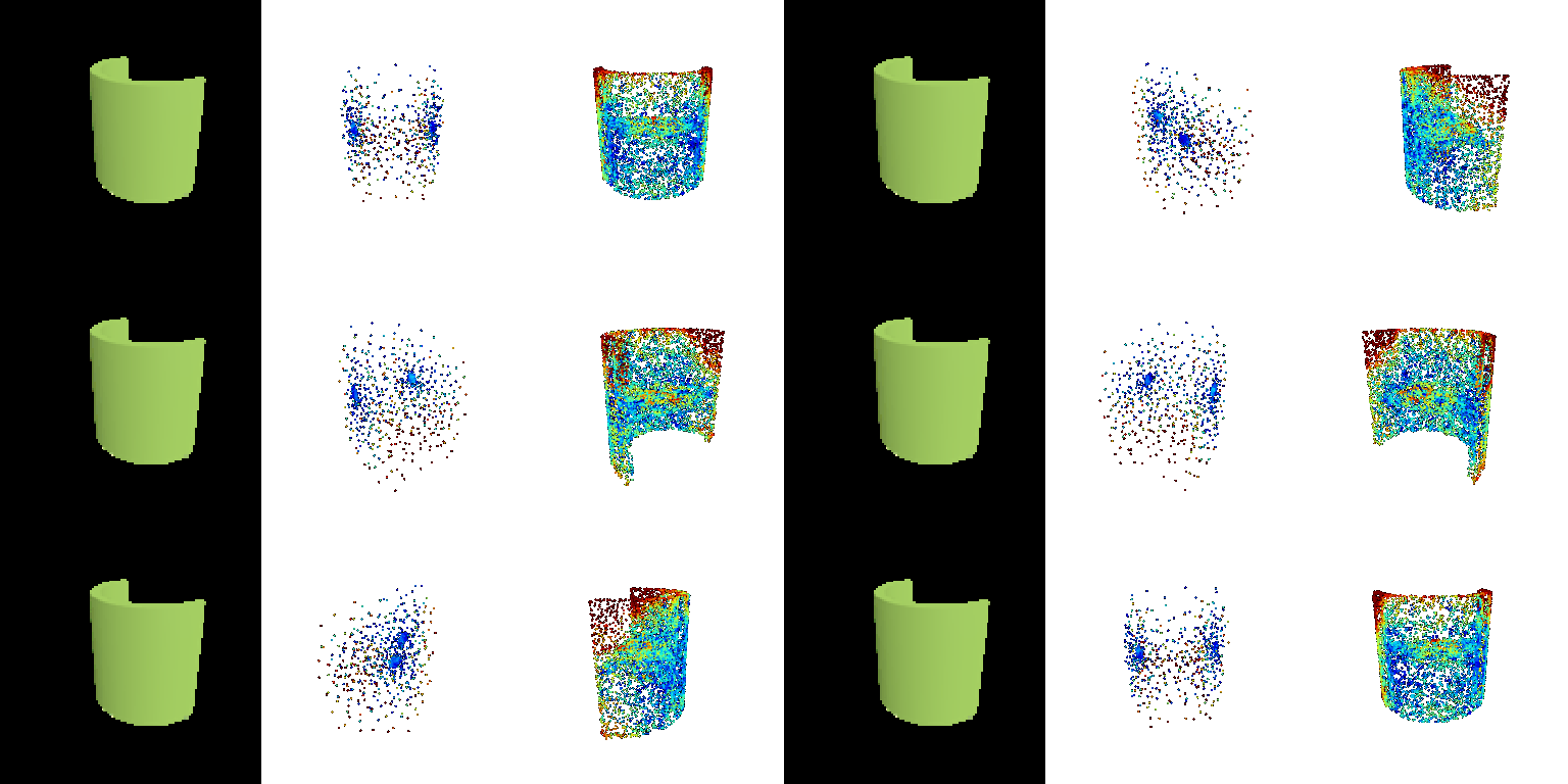
term costs accuracy.Where the point-cloud model is wrong. In the middle panel each predicted point is colored by its distance to the nearest ground-truth point, which is the precision side of F1. In the right panel each ground-truth point is colored by its distance to the nearest prediction, which is the recall side. Blue is 0; red is 0.1 or more, and F1 counts anything under 0.05.
Examples (input · prediction colored by error · GT colored by miss):
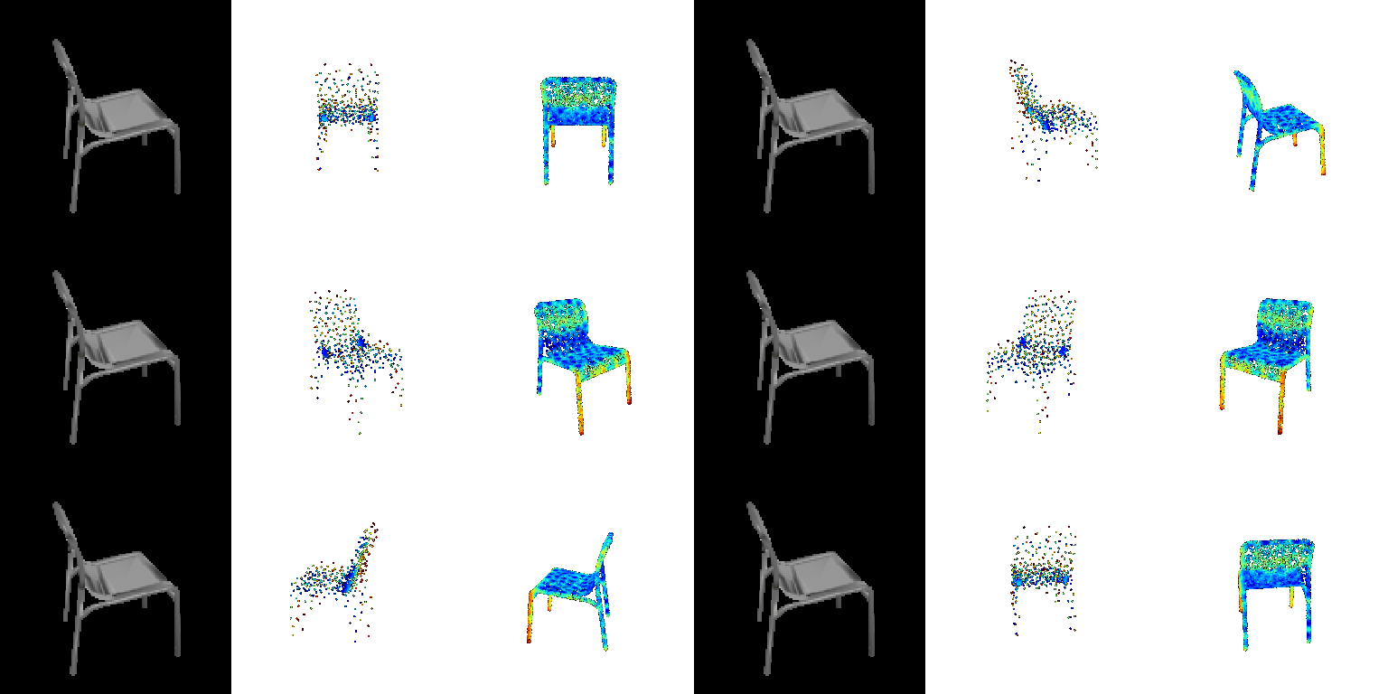
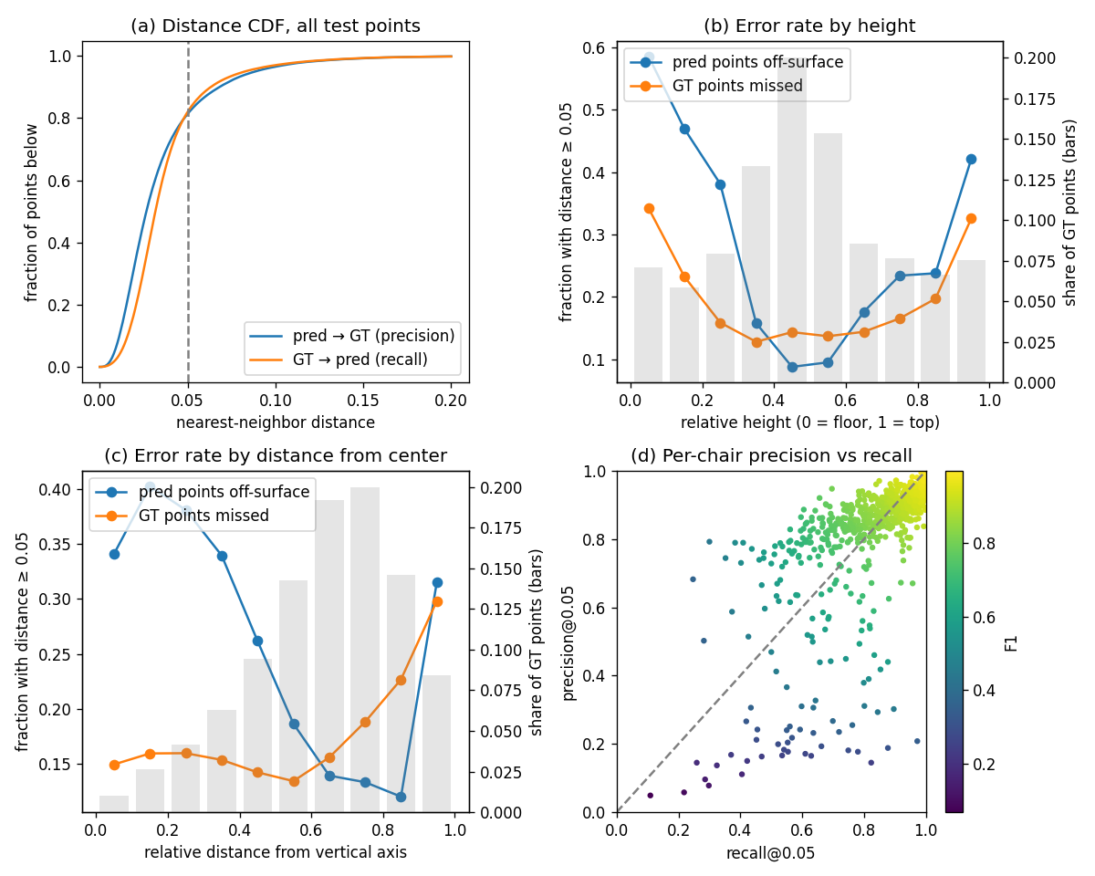
The same errors over the whole test set. Three chairs are anecdotes, so I pooled the per-point distances over every test chair (1000 predicted and 1000 GT points each). For position I normalized each point to its own GT chair: height runs from 0 (floor) to 1 (top), and radius is the distance from the vertical axis, from 0 (center) to 1 (outermost GT point). A point counts as an error when its distance is at least 0.05, the F1 threshold.
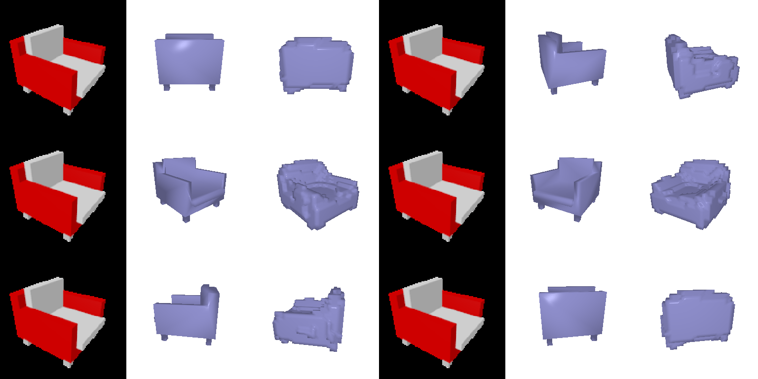
What the mesh latent space encodes. I encoded two
test images (a boxy armchair and a thin folding chair), linearly
interpolated their 512-d ResNet features and decoded each blend with the
w_smooth=1 mesh model from 2.4, which is the easiest to
read.

The shape changes gradually with no sudden jumps. As α goes from 0 to 1 the wide, low armchair body narrows, and the backrest and legs become taller and more separated, heading toward the folding chair. So the decoder maps nearby features to nearby shapes, which is a continuous shape space rather than a lookup of training chairs.
F1@0.05 = 50.0
An MLP takes the image feature and a 3D query point and returns an occupancy logit. At both training and test time it is queried on a fixed 32³ meshgrid in (-1, 1)³, then trained and evaluated exactly like the voxel model. Feature and coordinate are each projected to 128-d and summed. That is the same computation as one linear layer on their concatenation, but it avoids a 32×32768×515 input tensor. Three more 128-wide layers follow.
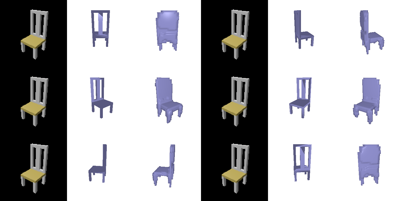
Examples (input · ground truth · prediction):
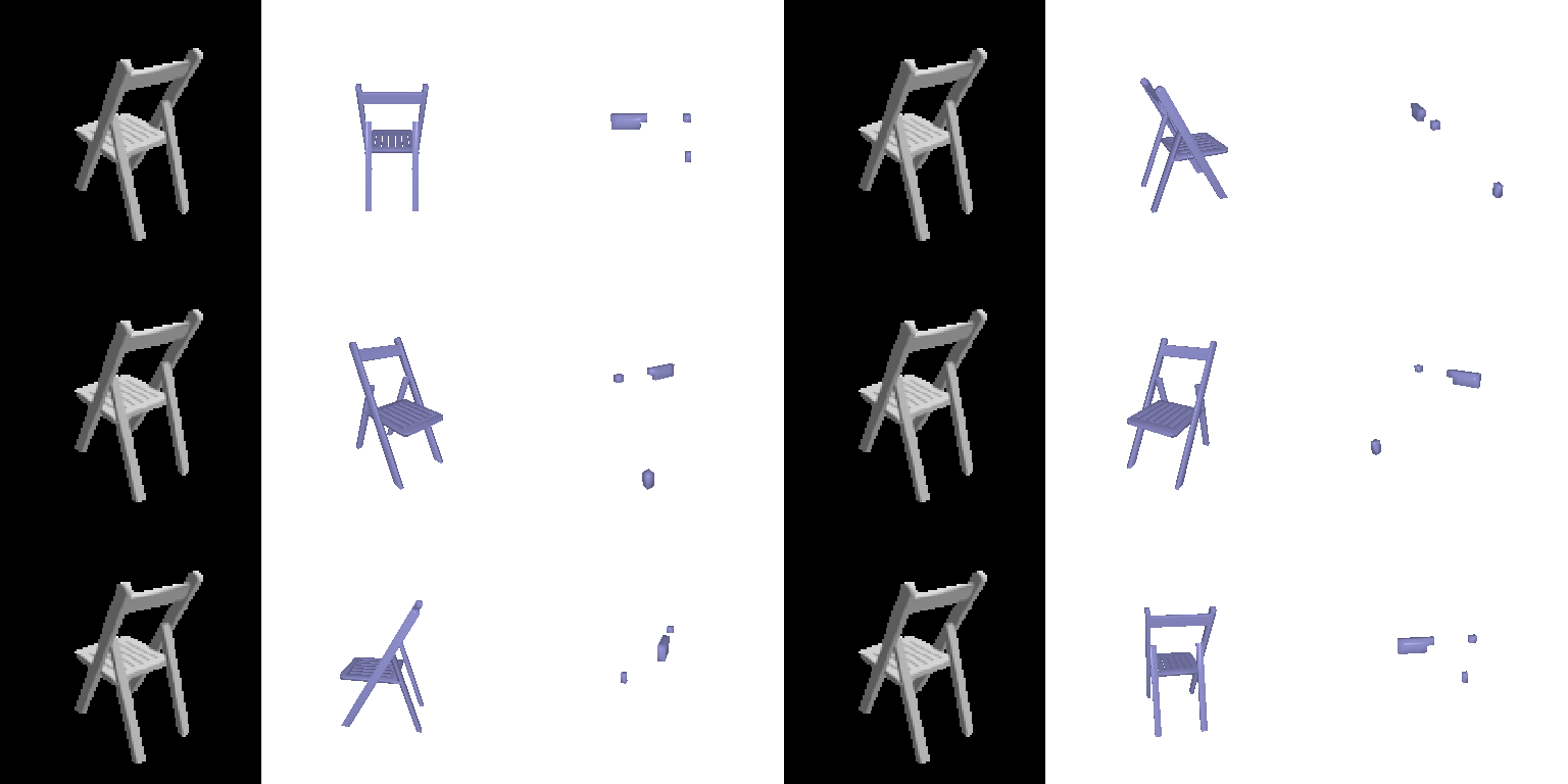
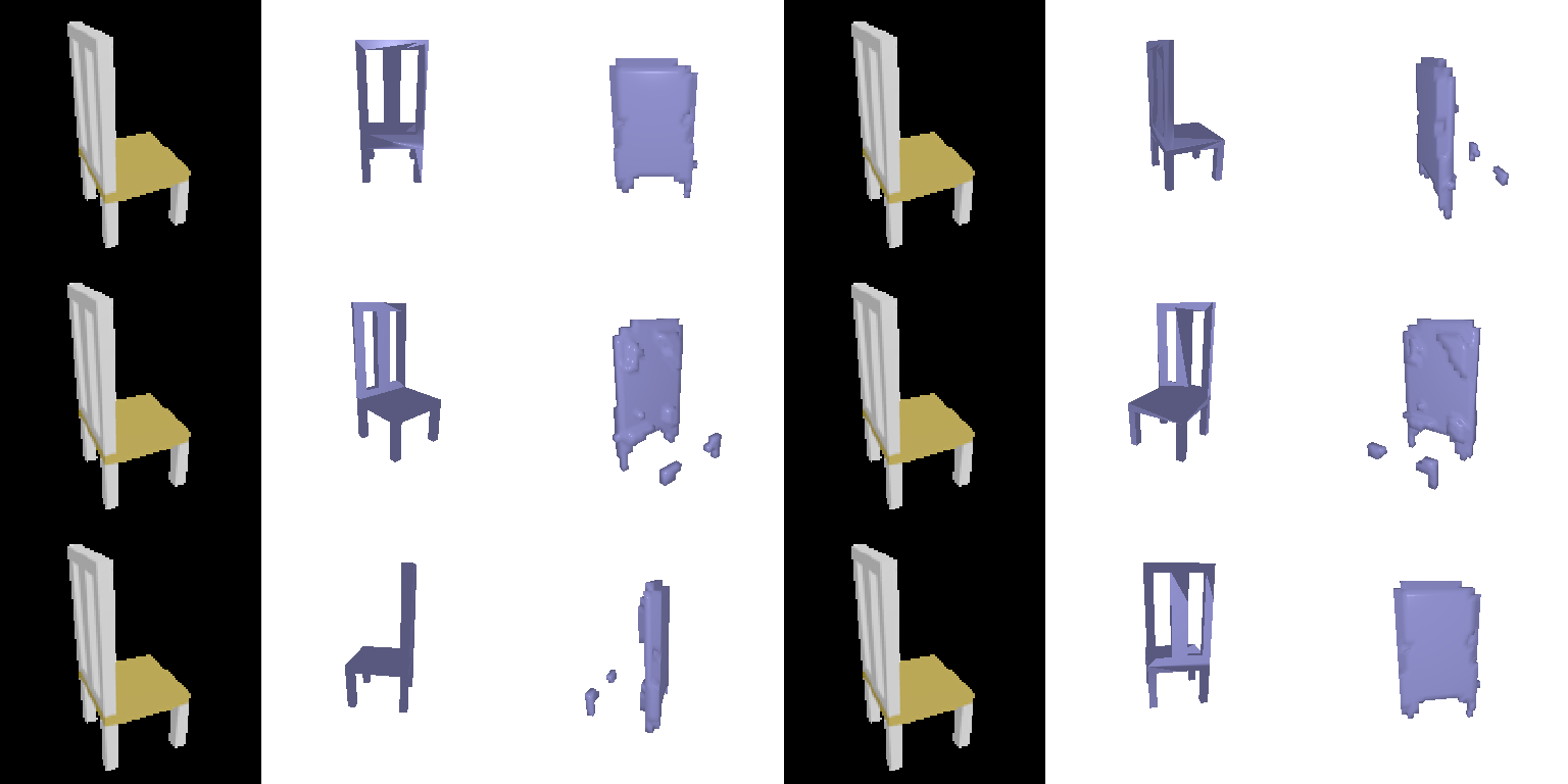
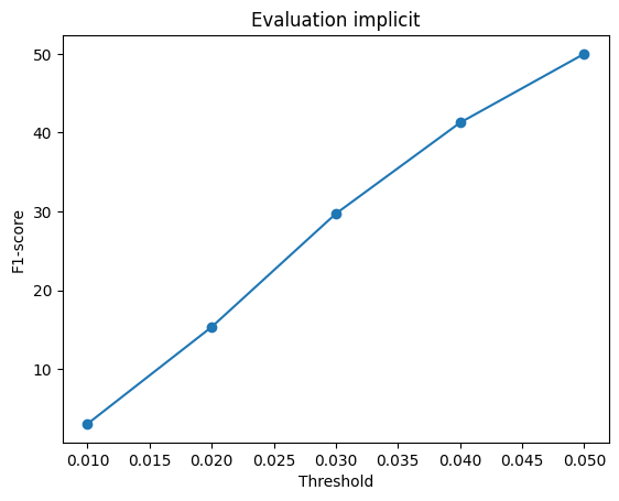
It is slightly below the convolutional voxel decoder (50.0 vs 54.9). It has the same empty-prediction problem, worse: 80 of 678 chairs come out empty. A plain MLP on raw xyz is biased toward low-frequency functions, and conditioning only the first layer on the image makes shapes too smooth to cross 0.5 on thin chairs. Unlike the voxel decoder, it can also be queried at any resolution.
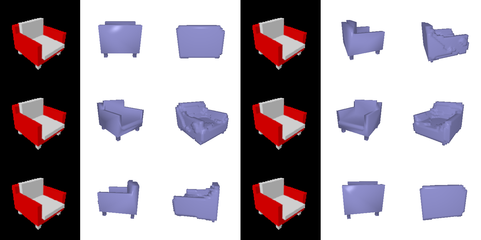
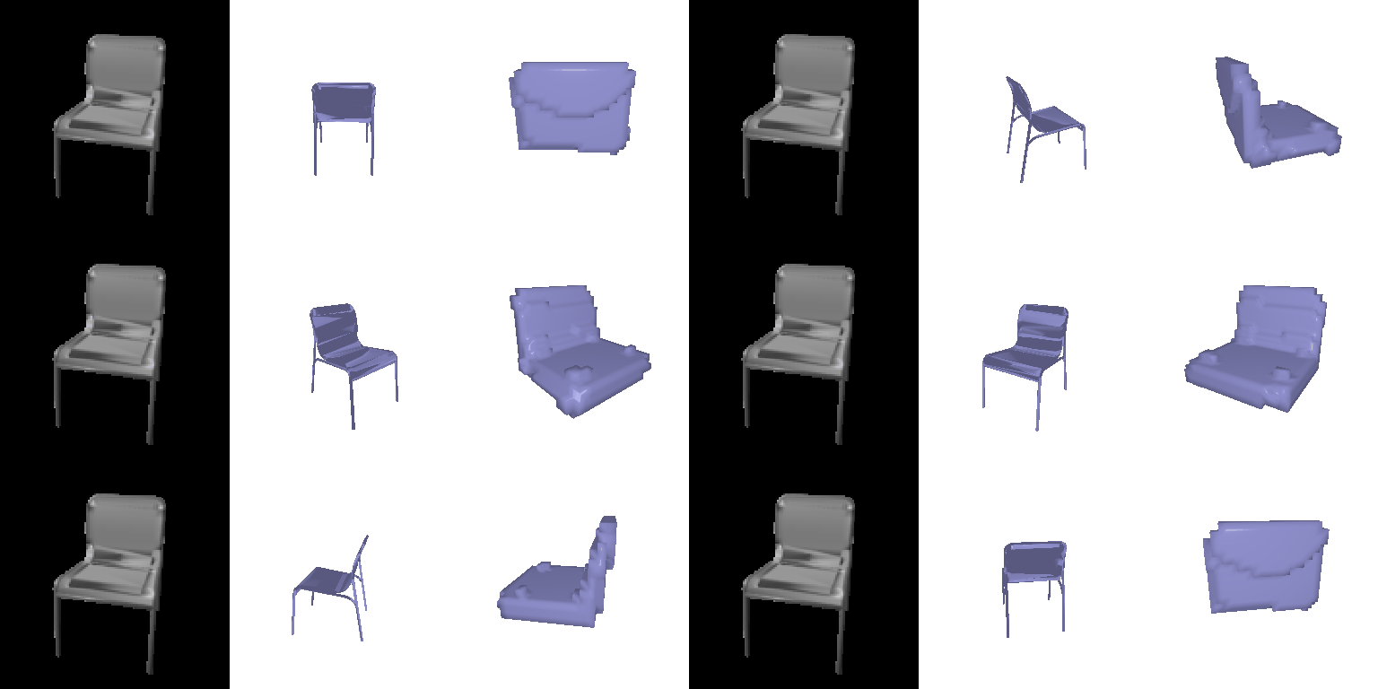
F1@0.05 = 55.2
To fix the weak conditioning I replaced the MLP with the decoder from Occupancy Networks (Mescheder et al., CVPR 2019). The query point goes through a linear layer to 256-d, then 5 ResNet blocks. Every normalization layer is a conditional batch norm, so its scale and shift are predicted from the image feature, and the image affects every layer instead of only the first. The decoder has 3.5M parameters. Training also follows the paper: each step queries 2048 random points from a box 10% larger than the grid, instead of the fixed 32³ grid. The paper checks whether each point is inside the true mesh. Only 32³ ground-truth voxels are available here, so each point takes the value of its nearest voxel, and the model cannot learn anything finer than a voxel. Evaluation queries the same 32³ grid as before, so the numbers are directly comparable; I did not implement the paper’s coarse-to-fine surface extraction.
Examples (input · ground truth · prediction):
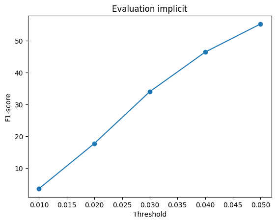
| Decoder | F1@0.05 | Empty predictions | F1 over non-empty chairs |
|---|---|---|---|
| Voxel (2.1) | 54.9 | 32 | – |
| MLP implicit | 50.0 | 80 | 56.7 |
| ONet implicit | 55.2 | 100 | 64.8 |
F1@0.05 = 75.0
An MLP maps the image feature, a random 2D sample (u, v) in [0, 1]² and a one-hot patch id (8 patches) to a 3D point. Each patch learns to fold a unit square onto part of the chair. The 1000 samples are redrawn every forward pass, and training uses the chamfer loss.
Examples (input · ground truth · prediction):
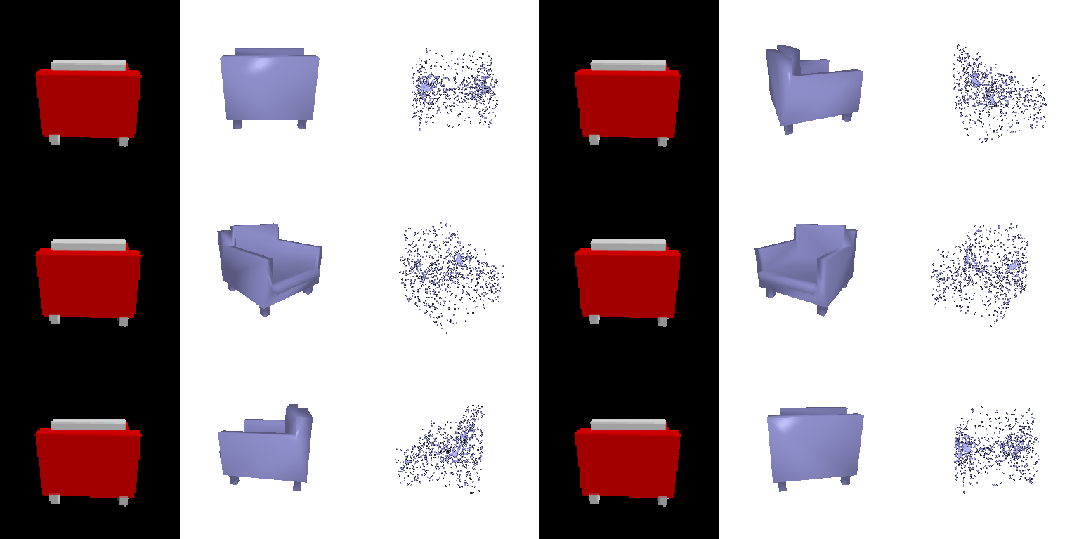
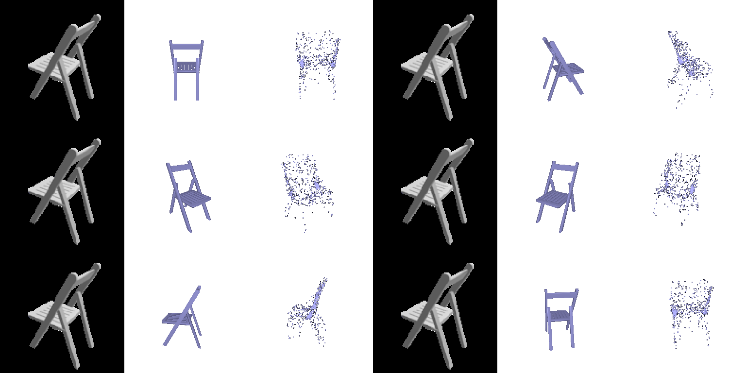
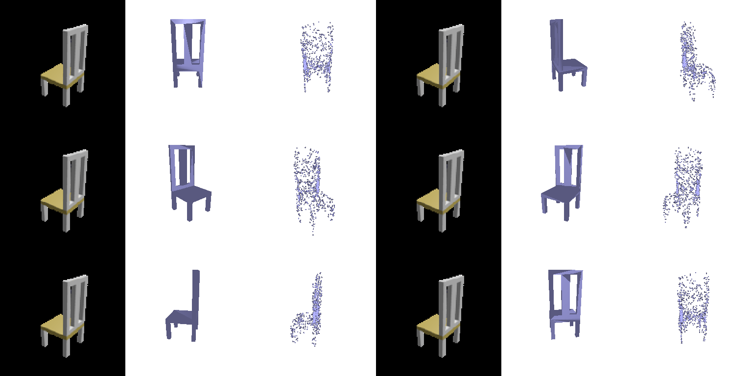
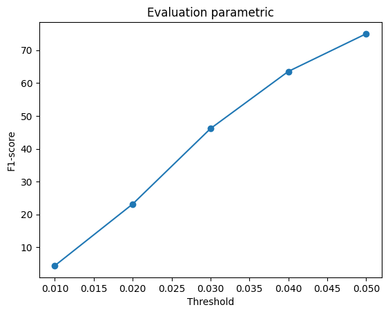
It lands between the mesh and the free point cloud. It can be sampled densely at any resolution, but the continuity of each patch makes it slightly less flexible than 1000 independent points, and resampling (u, v) every pass adds noise to training.
I retrained the point-cloud model from 2.2 on the three-class split
(split_3c.json: 3640 airplanes, 3146 cars, 6100 chairs for
training) with the same settings: 10k iterations, batch 32, chamfer
loss. Set R2N2_FULL=1 to switch
dataset_location.py to the extended dataset. Both models
are evaluated on the same three-class test set (405 airplanes, 368 cars,
678 chairs); the chair test models are the same 678 as in section 2.
| Trained on | Chair | Car | Airplane | All |
|---|---|---|---|---|
| Chair only (2.2 model) | 80.2 | 68.4 | 68.9 | 74.1 |
| Chair + car + plane | 79.8 | 93.3 | 96.2 | 87.8 |
F1@0.05 per test class.
Examples, chair-only model then three-class model on the same object (input · ground truth · prediction):
| Chair only | Three classes | |
|---|---|---|
| Airplane |  |
 |
| Car |  |
 |
| Chair |  |
 |
Chairs: no change. 80.2 vs 79.8 is within run-to-run noise. Each eval picks a random view per object, and the same chair-only checkpoint has scored 79.2, 80.0 and 80.2 on different runs. Adding two classes did not help chairs and did not hurt them, even though chairs are only 47% of the three-class training set. With the same 10k iterations, the three-class model sees each chair about half as often (about 25 epochs of the larger set vs 52 of the chair set), and it still matches.
Cars and airplanes: large gain. The chair-only model has only one shape prior, so it turns a car or a plane into a chair-shaped cloud: a compact, tall blob. It still scores 68–69 because the normalized objects overlap in the bulk of their volume, and F1@0.05 counts any point within 5% of the object size. The three-class model produces class-appropriate shapes: flat and spread out for airplanes, a long low box for cars.
Why cars and planes score higher than chairs. Within each class, cars are compact boxes and airplanes share one layout (fuselage, two wings, tail). Chairs vary much more in structure: legs vs a solid base, slats, arms, open or closed backs. A regression decoder trained with chamfer tends toward a per-class average shape, and that average is a good answer for cars and planes but a poor one for thin chair parts.
Consistency and diversity. The chair-only model’s outputs for non-chairs look alike regardless of input, which shows that its output space covers only chairs. The three-class model first recognizes the class from the image and then refines within it. Its chair predictions look the same as the chair-only model’s, so the extra classes add diversity across categories without spreading the chair predictions out.
model.obj. Caching parsed verts and
faces as model.pt and decoding only the sampled view (not
all 24) brought it to about 0.03 s per batch.--load_feat. All models train on the GPU
from raw images.