Assignment 2 — Single View to 3D
16-825: Learning for 3D Vision
1. Exploring loss functions
1.1 Fitting a voxel grid
def voxel_loss(voxel_src, voxel_tgt):
    loss = torch.nn.functional.binary_cross_entropy_with_logits(voxel_src, voxel_tgt)
    return loss
1.2 Fitting a point cloud
def chamfer_loss(point_cloud_src, point_cloud_tgt):
    dist_src = knn_points(point_cloud_src, point_cloud_tgt, K=1).dists  # b x n_src x 1
    dist_tgt = knn_points(point_cloud_tgt, point_cloud_src, K=1).dists  # b x n_tgt x 1
    loss_chamfer = dist_src.squeeze(-1).mean(dim=1) + dist_tgt.squeeze(-1).mean(dim=1)
    return loss_chamfer.mean()
1.3 Fitting a mesh
def smoothness_loss(mesh_src):
    loss_laplacian = mesh_laplacian_smoothing(mesh_src, method="uniform")
    return loss_laplacian
2. Reconstructing 3D from a single view
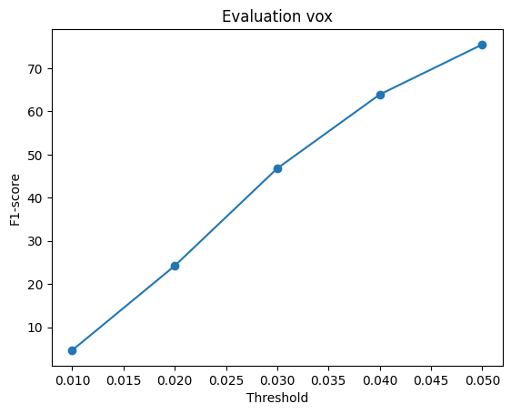
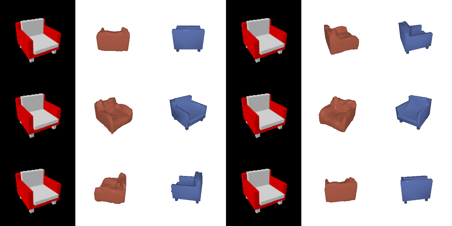
2.1 Image to voxel grid
F1@0.05 on the chair test set (678 models): 75.50


2.2 Image to point cloud
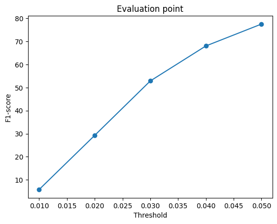
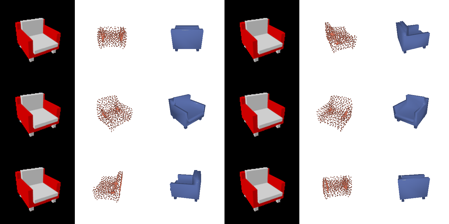
F1@0.05 on the chair test set (678 models): 77.48
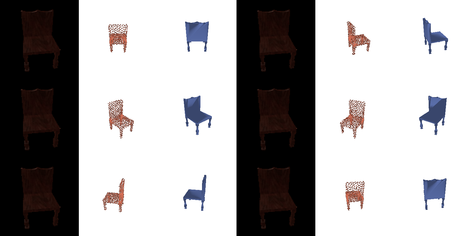
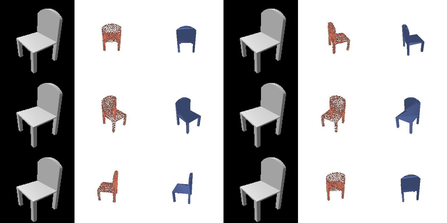
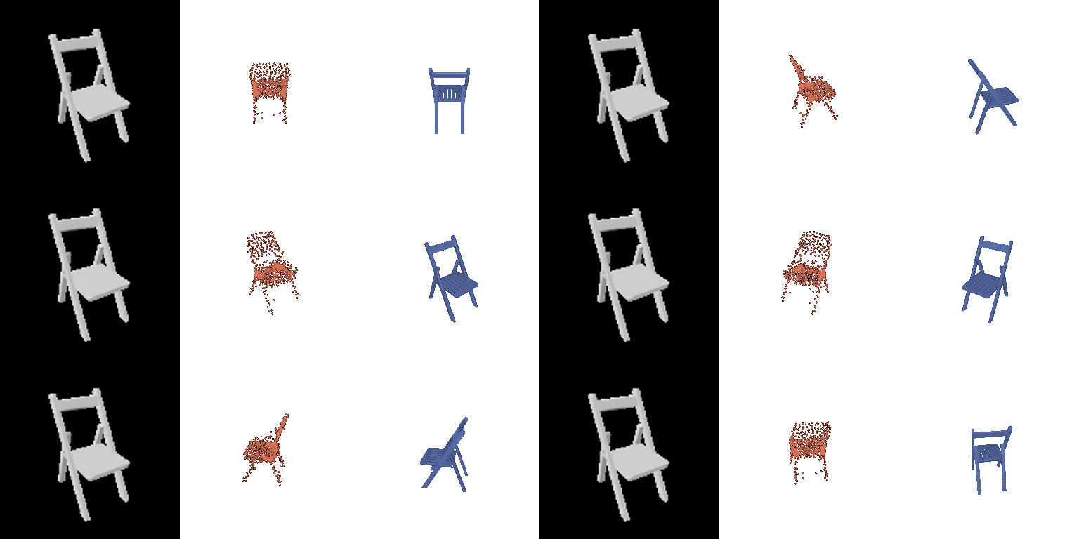
2.3 Image to mesh
F1@0.05 on the chair test set (678 models): 74.08
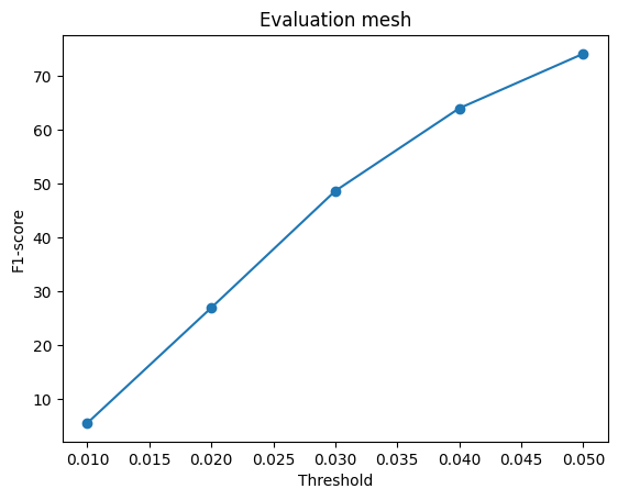
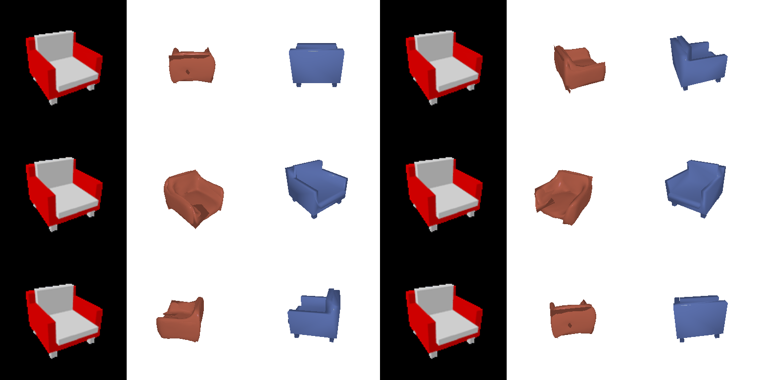

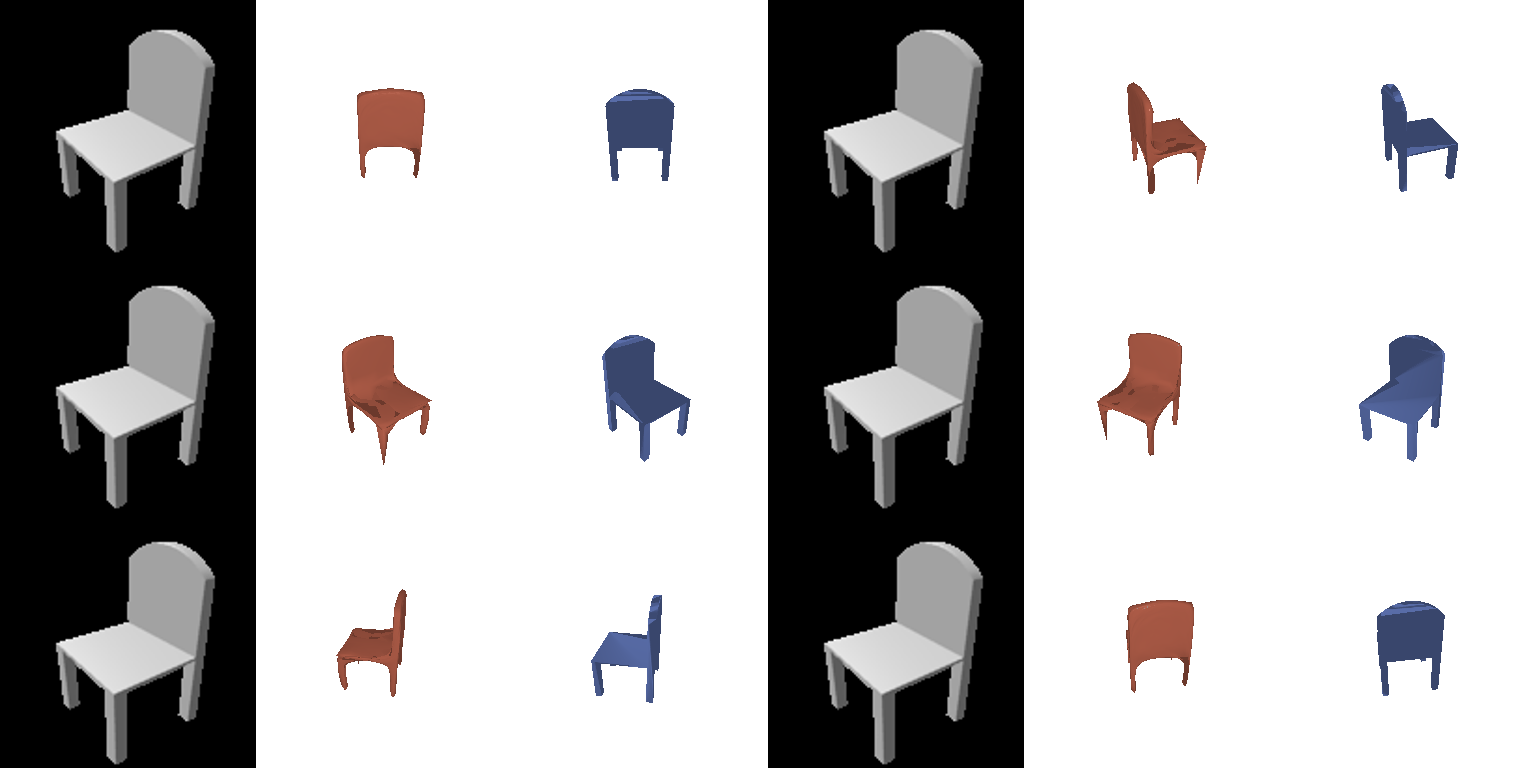
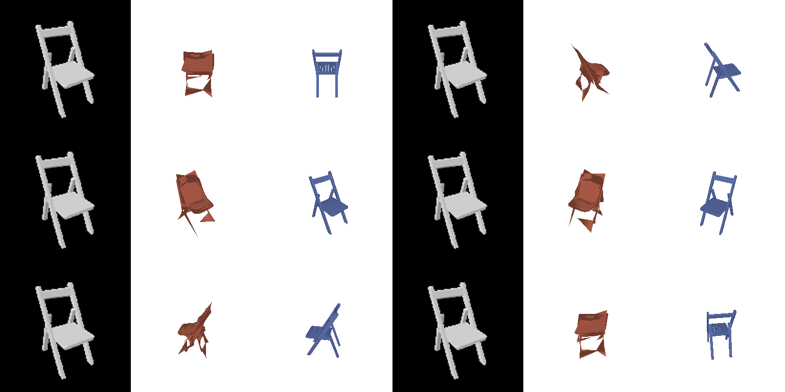
Comparing voxels, point clouds and meshes
| Representation | F1@0.05 |
|---|---|
| Point cloud (2.2) | 77.48 |
| Voxel grid (2.1) | 75.50 |
| Mesh (2.3) | 74.08 |
The point cloud does best because its points can go anywhere, and chamfer loss is basically what F1 measures. Voxels lose thin parts like legs to the 323 grid. The mesh is lowest because it starts from one sphere, so it can't open holes between legs, and smoothing pulls thin parts inward. Still, the mesh is the only one that gives a real surface.
2.4 Effect of the smoothness weight (w_smooth)
I test the effect of the Laplacian smoothness weight on the 2.3 mesh decoder, training it with w_smooth = 0, 0.1, 1 and 10.
| w_smooth | F1@0.02 | F1@0.05 |
|---|---|---|
| 0 | 26.39 | 75.07 |
| 0.1 (default) | 25.65 | 73.23 |
| 1 | 24.41 | 71.58 |
| 10 | 18.10 | 59.33 |
The same test chair (sample 400) at each weight:


F1@0.05 drops from 75.1 to 73.2, 71.6 and finally 59.3 since the Laplacian term keeps pulling each vertex toward its neighbours, and thin parts like the legs get squeezed away first. Turning smoothing off gives the best number, but the mesh itself looks broken. F1 only checks point distances, but not penalize folded, self-intersecting faces. I think 0.1 is the sweet spot: it cleans up the surface and costs less than 2 points of F1.
2.5 Interpreting the models
Parametric charts coloured by patch
This visualization shows the 3.2 parametric prediction from four viewpoints, next to the input image. The decoder builds the point cloud from 4 learned 2D charts, and each of the 4,000 sampled points is coloured by the chart that produced it (red, blue, green or orange).


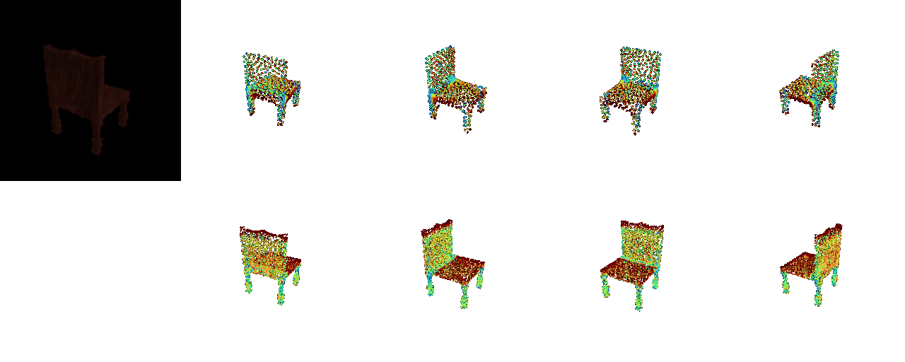
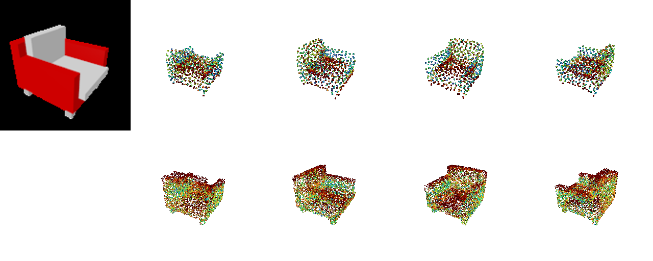
Point cloud error heatmaps
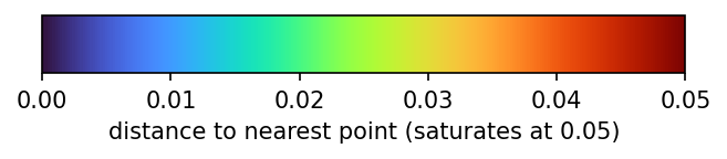
This visualization colours the 2.2 point cloud prediction by error. The top row shows each predicted point coloured by its distance to the ground truth (precision errors), and the bottom row shows each ground-truth point coloured by its distance to the prediction (missed regions). The colour scale saturates at 0.05, the F1 threshold, so dark red means the point is counted as wrong.
Interpolating between two chairs
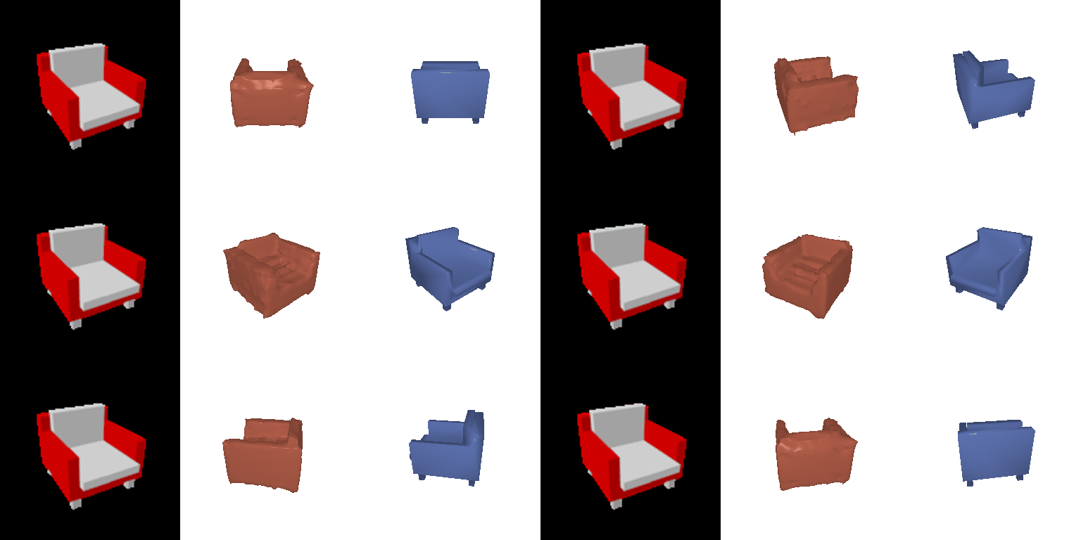
This visualization blends the ResNet features of two test images with weights 0, 0.25, 0.5, 0.75 and 1, and decodes each blend with the 3.1 implicit decoder, showing how one chair turns into the other.

3. Exploring other architectures / datasets
3.1 Implicit network
An MLP takes the image feature and a positionally encoded 3D point and outputs its occupancy logit. It is trained on 4,096 sampled points per shape with BCE, then queried on a 323 grid over (-1,1)3 and meshed with marching cubes.
F1@0.05 on the chair test set (678 models): 76.82 (voxel decoder: 75.50)
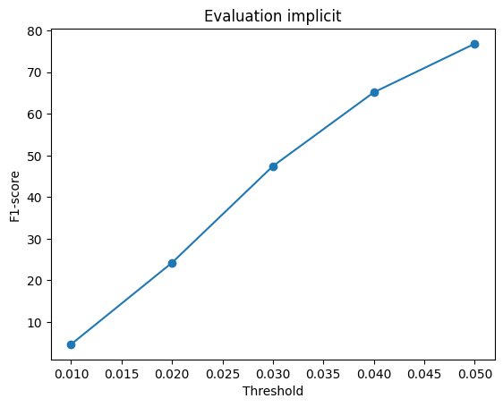
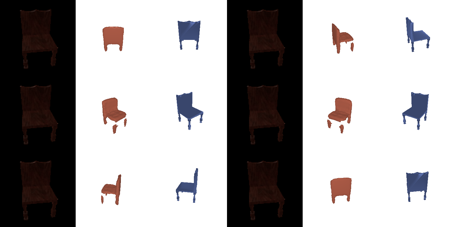
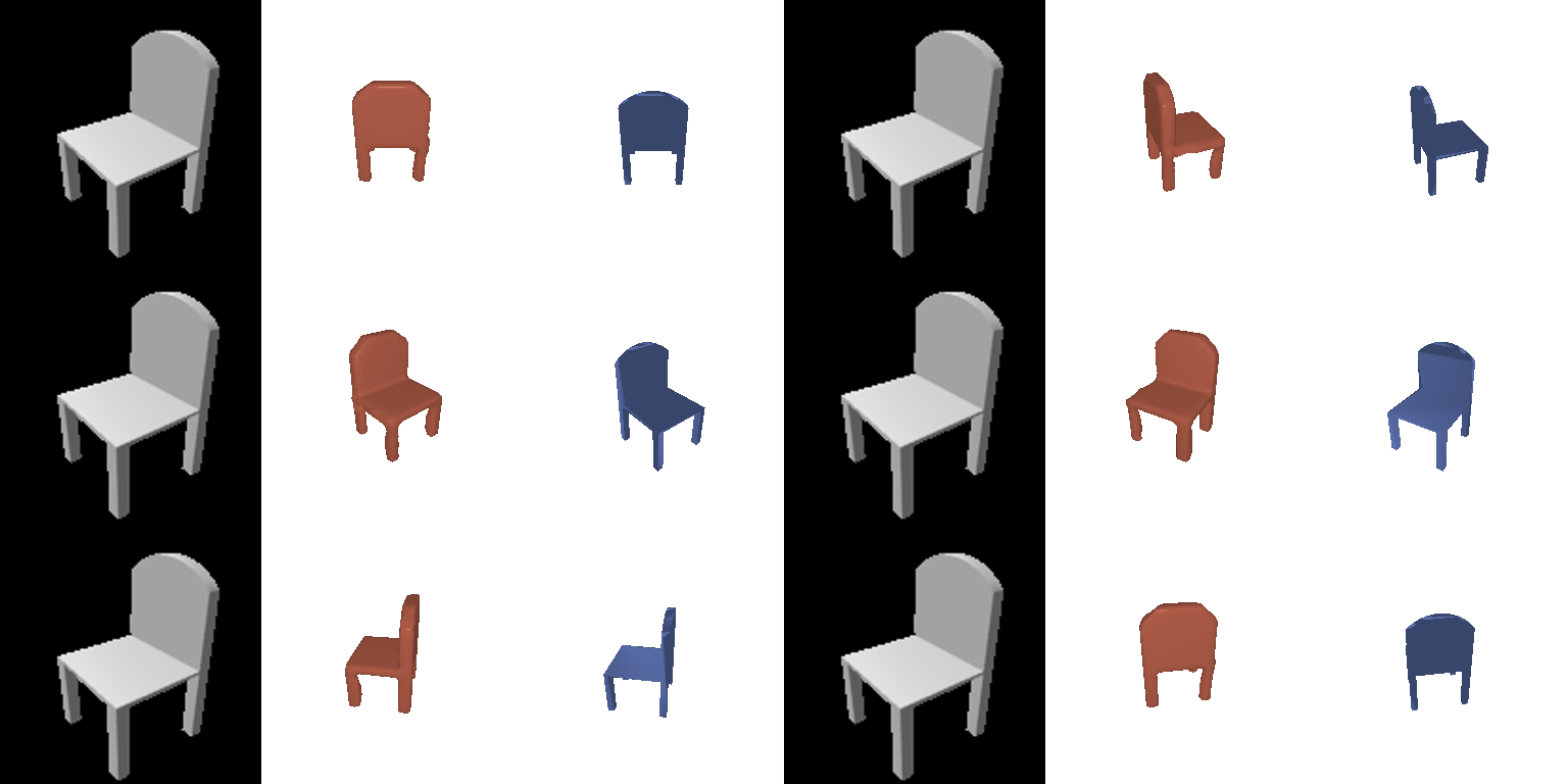
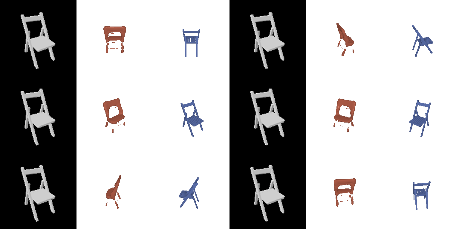
The implicit network beats the voxel decoder by a little (76.82 vs. 75.50). One MLP is shared across all 3D points, so the predicted shape comes out smoother. The gain is small because I still mesh it at 323, but I could query it at a higher resolution without retraining.
3.2 Parametric network
4 per-chart MLPs map random (u, v) points in [0,1]2, combined with the image feature, to 3D points (250 each, 1,000 total), trained with chamfer loss.
F1@0.05 on the chair test set (678 models): 75.26 (point decoder: 77.48)
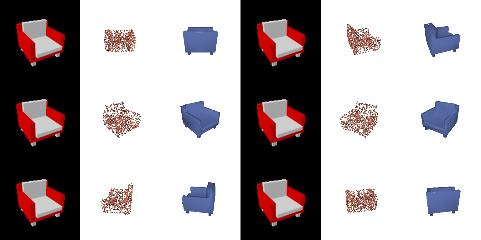
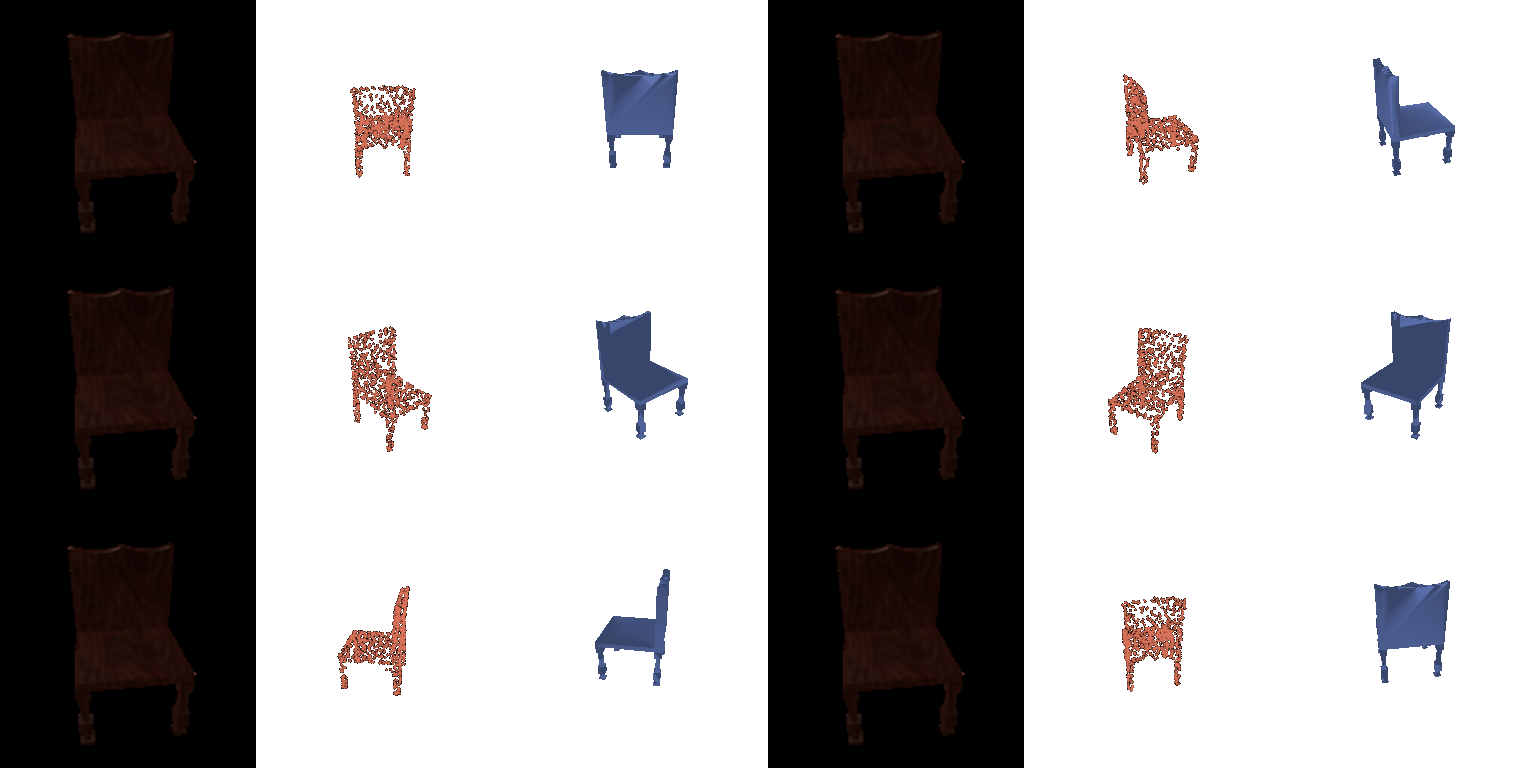
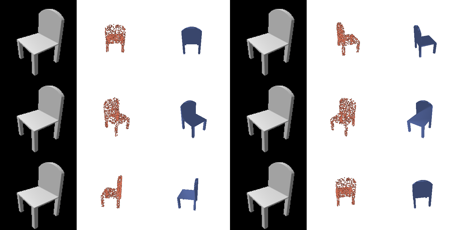
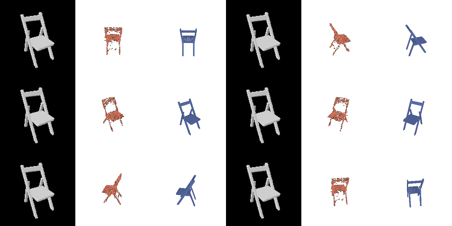
The parametric network is slightly worse than the plain point decoder (75.26 vs. 77.48). Each chart has to be a smooth surface bent from a square, so it has to stretch over thin legs and gaps, and points there miss the surface. In return, the output is more organised (each chart covers one part, see 2.5), and I can sample as many points as I want.
3.3 Extended dataset for training
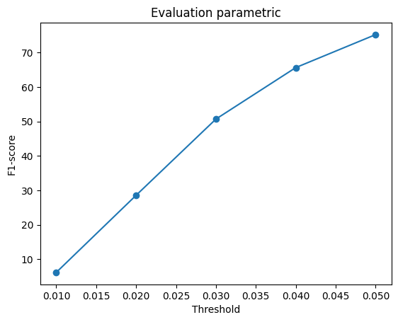
The 2.2 point decoder is trained on chairs only and on chairs + cars + planes, then both are tested on the same 678 chair test views.
| Trained on | F1@0.01 | F1@0.02 | F1@0.03 | F1@0.04 | F1@0.05 |
|---|---|---|---|---|---|
| Chairs only | 5.87 | 29.68 | 53.47 | 68.44 | 77.62 |
| Chair + car + plane | 4.72 | 26.28 | 51.16 | 67.37 | 77.25 |
The three-class model on all three test classes, F1@0.05:
| Class | Test models | F1@0.05 |
|---|---|---|
| Plane | 405 | 95.65 |
| Car | 368 | 92.25 |
| Chair | 678 | 77.58 |


The same chair test views, predicted by both models:


Car and plane predictions from the three-class model:

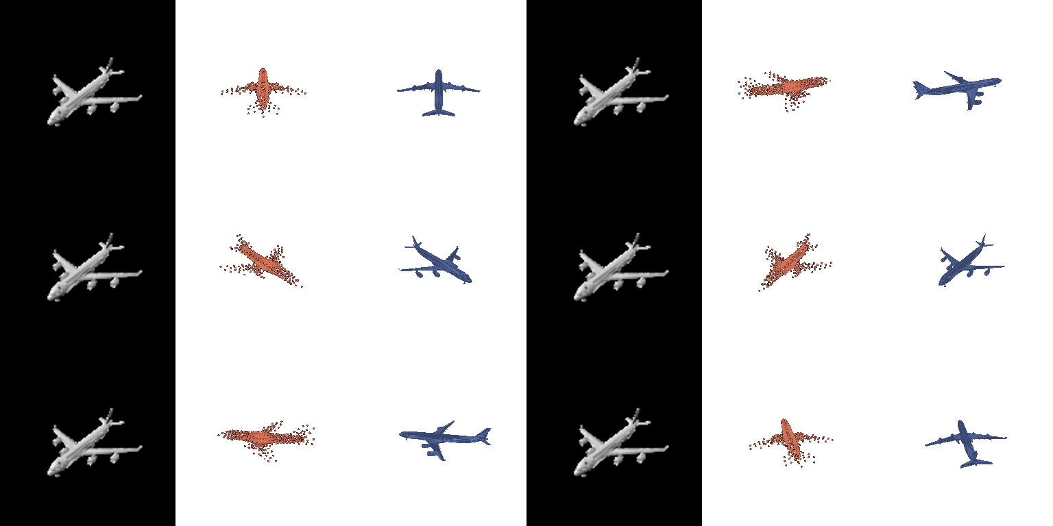
Adding cars and planes barely changes chair F1@0.05 (77.62 vs. 77.25), but the gap grows at tighter thresholds (29.7 vs. 26.3 at 0.02). So the model still gets the overall chair shape right, just less precisely. Its chairs look a bit noisier, but they never look like cars or planes, since the image makes the class obvious. I think this is because the decoder now has to cover three very different shape families and sees fewer chairs. Cars and planes score much higher (92 and 96) because their shapes are simpler, with no thin legs or holes.