16-825 Assignment 1: Rendering Basics with PyTorch3D
1. Practicing with Cameras
1.1 360-degree Renders
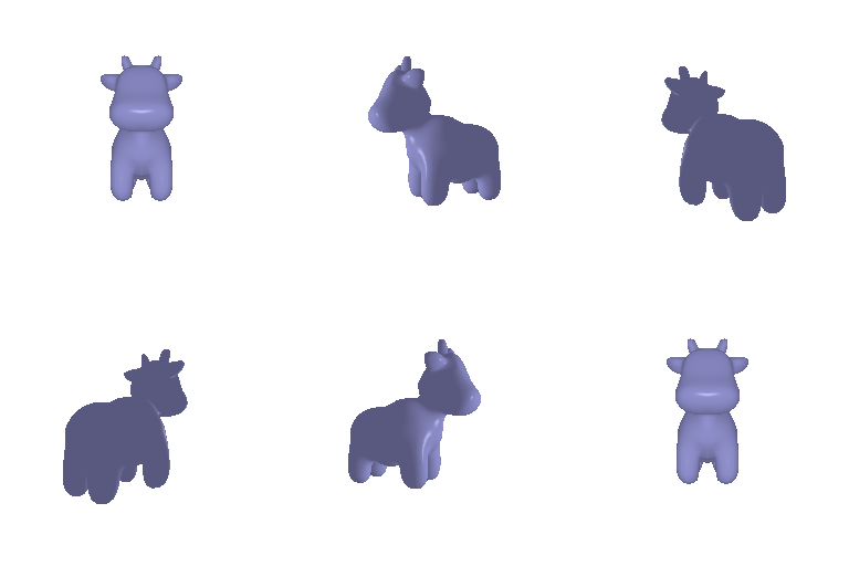
For the turntable, I kept the camera 3 units away at zero elevation and moved the azimuth 10° each frame.
look_at_view_transform gives me the R and T for every view, and I saved the
frames as a gif.
1.2 Re-creating the Dolly Zoom
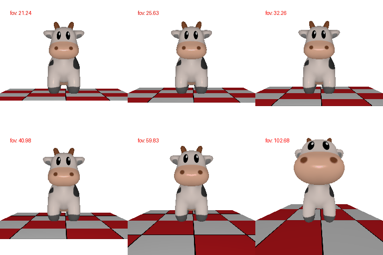
The key idea is that the cow should stay the same size while the field of view changes. I moved the camera
evenly from 8 units away to 1.2 units away. For each distance d, I picked the field of view that keeps
a 3-unit-wide region at the cow filling the same part of the frame: fov = 2·atan(3 / (2·d)).
The field of view goes from about 21° to about 103°. The cow barely changes, but the floor behind it
stretches out, which gives the Vertigo effect.
2. Practicing with Meshes
2.1 Constructing a Tetrahedron
I built a regular tetrahedron. Three vertices form an equilateral triangle on the y = 0 plane, and
the fourth one sits above them at (0, 1.633, 0). Each face is a triangle made of three of those vertices.
Vertices: 4 | Triangle faces: 4

2.2 Constructing a Cube
The cube's corners are at (±1, ±1, ±1). A triangle mesh can't hold a square
directly, so I split each of the 6 sides into 2 triangles.
Vertices: 8 | Triangle faces: 12
3. Re-texturing a Mesh
I chose color1 = [0, 0, 1] (blue) for the front of the cow and color2 = [1, 0, 0] (red)
for the back. For each vertex, I work out how far along the cow it is from front to back,
alpha = (z - z_min) / (z_max - z_min), and mix the two colors:
color = alpha·color2 + (1 - alpha)·color1. The head comes out blue, the middle turns
purple, and the tail is red.

4. Camera Transformations
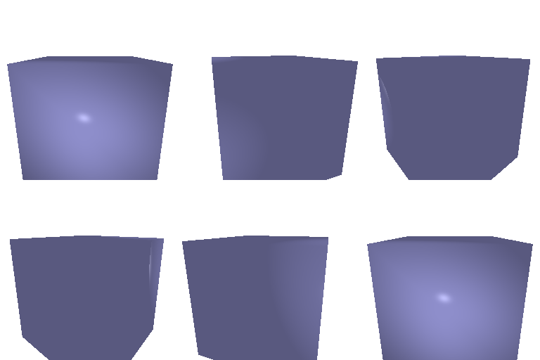
The starting camera has R_0 = [[1,0,0],[0,1,0],[0,0,1]] and T_0 = [0, 0, 3]. For each
target image, I found an R_relative and T_relative. The new camera then uses
R = R_relative @ R_0 and T = R_relative @ T_0 + T_relative.
| Target | R_relative | T_relative | Description |
|---|---|---|---|
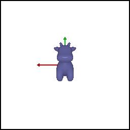
| Transform 1 | [[0,1,0],[-1,0,0],[0,0,1]] |
[0,0,0] |
The camera stays where it is but rolls 90° around the direction it's looking in. That's why the cow looks like it's lying on its side. |
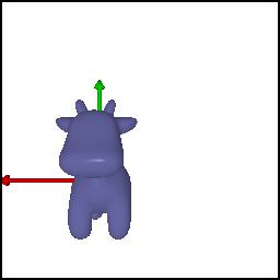
| Transform 2 | [[1,0,0],[0,1,0],[0,0,1]] |
[0,0,3] |
No rotation. The camera just backs up 3 more units, from 3 to 6 units away, so the cow looks smaller. |
| Transform 3 | [[0.985,0,0.174],[0,1,0],[-0.174,0,0.985]] |
[0,0,0] |
The camera turns 10° around the vertical axis. The cow moves off-center and we see it from a slightly different angle. |
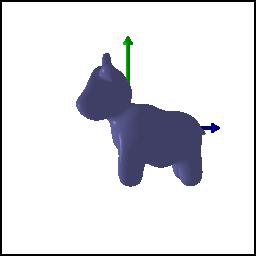
| Transform 4 | [[0,0,1],[0,1,0],[-1,0,0]] |
[-3,0,3] |
The camera turns 90° around the vertical axis so it sees the cow from the side. If I only rotated,
T would become [3,0,0] and the cow would be out of view. Adding
T_relative = [-3,0,3] brings it back to T = [0,0,3], 3 units in front of the camera. |


5. Rendering Generic 3D Representations
5.1 Rendering Point Clouds from RGB-D Images
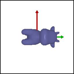
I turned each RGB-D image into a point cloud with unproject_depth_image, keeping only the pixels
inside the plant mask. Some pixels in the mask have no depth reading (depth = 0), and those turn into
NaN points, so I dropped them too. Both point clouds are already in world coordinates, so to get the union I just
stacked them together. For the turntable, the camera circles the plant 6 units away. I also flipped the camera's
up direction, because otherwise the plant renders upside down.


5.2 Parametric Functions
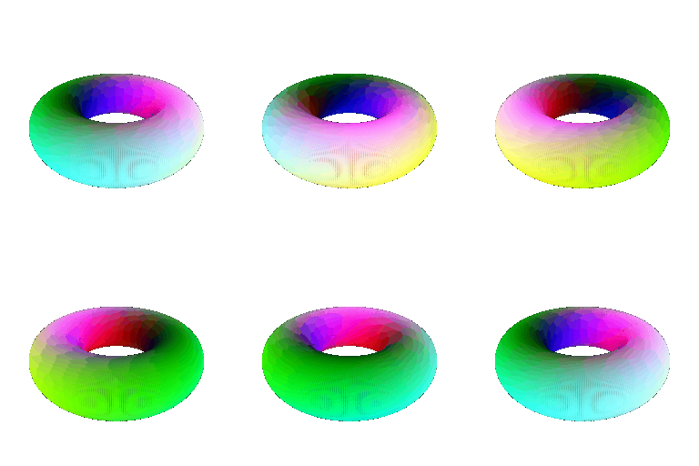
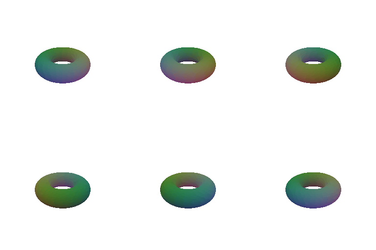
Torus. I used a big radius R = 1.0 and a tube radius r = 0.4, and sampled
θ and φ on a 400×400 grid:
x = (R + r cos θ) cos φ
y = r sin θ
z = (R + r cos θ) sin φ
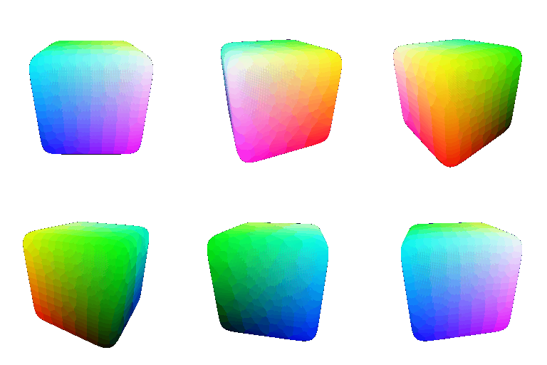
My own object: a rounded cube (superquadric). I started by sampling a 130×130 grid on each of the 6
sides of a cube. Then I divided every point by its L10 norm, which pulls it onto the surface
|x|¹⁰ + |y|¹⁰ + |z|¹⁰ = 1. The result is a cube with softened edges.
In both shapes, each point's color comes from its position.
5.3 Implicit Surfaces
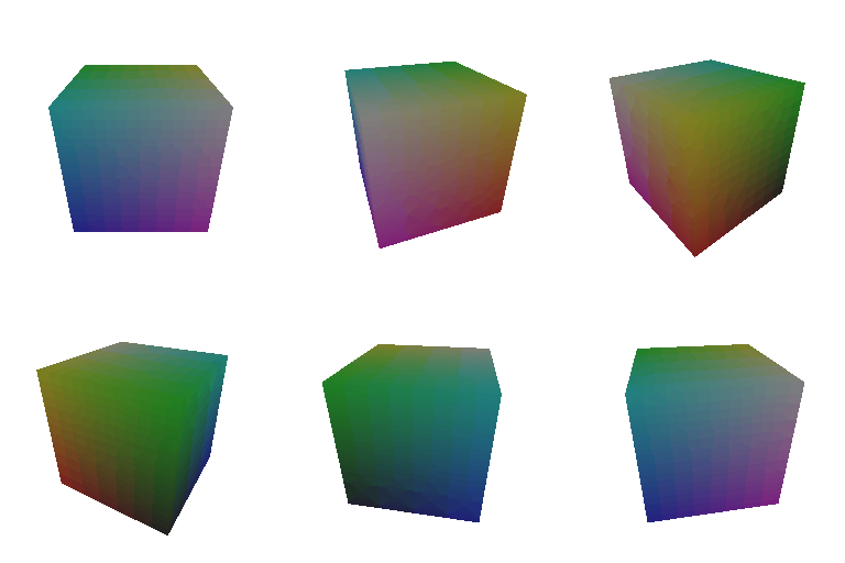
For each shape, I evaluated its function on a 64×64×64 grid covering [-1.1, 1.1] in every
direction. Then I ran marching cubes (mcubes) to pull out the surface where the function equals zero,
and scaled the vertices from grid indices back to world coordinates. I attached the light to the camera, so the side
facing us is always lit.
- Torus:
F(x,y,z) = (√(x² + z²) - R)² + y² - r², withR = 0.7andr = 0.3 - My own object, a cube:
F(x,y,z) = max(|x|, |y|, |z|) - 1
Mesh vs. point cloud: tradeoffs
- Quality: Meshes look solid and can be lit properly. Point clouds are just dots, so you see gaps unless you use a lot of them.
- Speed: A mesh covers the surface with fewer primitives. My torus point cloud needed 160k points, and marching cubes gets slow as the grid gets finer.
- Memory: Points only store positions and colors, but you need many of them. A mesh also stores faces, but it's usually more compact for the same look.
- Ease of use: Point clouds are easier to make and merge (5.1 was a single concatenation). Meshes need correct faces, though marching cubes builds them for you.
6. (Extra Credit) Do Something Fun
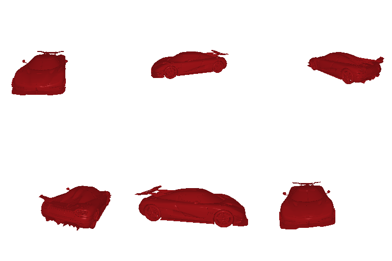
I wanted to try something much heavier than the cow, so I downloaded a detailed Koenigsegg sports car model and rendered a 360° turntable of it. The first render looked wrong: the OBJ file held the whole studio scene, not just the car, including area lights and a huge background sheet. Blender saves objects in order, so I kept only the first 752,508 vertices (the car) and the faces that use them, then moved the car to the origin.
The car has about 1.5 million faces, which took two more fixes:
- With the default settings, pieces of the car went missing from the frame. PyTorch3D sorts faces into screen
bins, and too many faces landed in the same few bins, so I raised
max_faces_per_binto 200,000. - I attached the light to the camera, so the car stays lit the whole way around.
7. (Extra Credit) Sampling Points on Meshes
To sample points evenly over the cow's surface, I do three steps for every point:
- Pick a face. Bigger triangles should get more points, so I compute each face's area,
½‖(v1-v0) × (v2-v0)‖, and pick faces with probability proportional to area usingtorch.multinomial. - Pick a spot on that face. I draw
αandα2uniformly from [0, 1] and setα1 = 1 - √α. The square root matters: ifα1were drawn uniformly, points would pile up in one corner of the triangle. - Compute the point:
p = α1p1 + (1-α1)α2p2 + (1-α1)(1-α2)p3.
In each gif, the original cow mesh is on the left and the sampled point cloud is on the right. With 10 or 100 points you can only guess the shape, at 1,000 the cow is recognizable, and at 10,000 it's almost solid.


