
henrytsu · 16-825 · Assignment 3
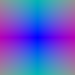
| Pixel coordinates | Ray directions |
|---|---|
|
|
64 uniformly spaced samples per ray.
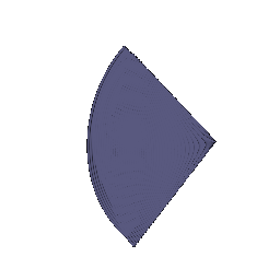
20 views at 256 × 256. Depth is normalized by its maximum value.
| Spiral rendering | Normalized depth |
|---|---|
 |
 |
| Optimized parameter | Value (rounded to two decimal places) |
|---|---|
| Center | (0.25, 0.25, 0.00) |
| Side lengths | (2.01, 1.50, 1.50) |

Lego, 128 × 128, 250 epochs. The position MLP has six 128-unit layers, six encoding frequencies, and a skip connection at layer 3. Density uses ReLU; color uses sigmoid.
| Setting | Value |
|---|---|
| Rays per iteration / samples per ray | 1,024 / 128 |
| Near / far | 2.0 / 6.0 |
| Initial learning rate | 0.0005 |
| Learning-rate multiplier | 0.8^(epoch / 50) |
| Loss | RGB MSE |

Viewing direction, encoded with two harmonic frequencies, is added to the color branch. Density depends only on position.
Both materials models use 250 epochs, 128 × 128 images, 1,024 rays per iteration, 128 samples per ray, near/far bounds of 1.0/7.0, and an initial learning rate of 0.0001.
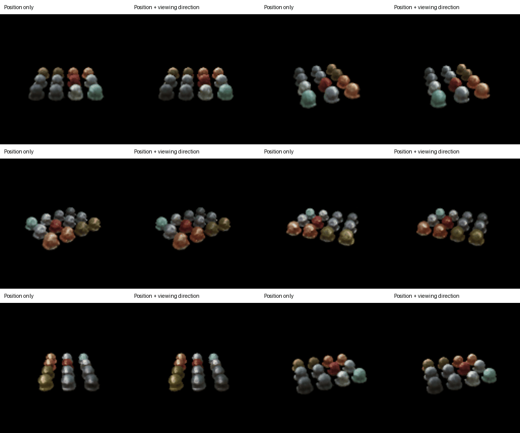
Left: position only. Right: position + viewing direction. Cameras and animation frames match.
| Frame 0 | Frame 5 |
|---|---|
 |
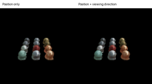 |
The differences are subtle, mainly in brightness and highlights; reflections remain blurred. View dependence can represent reflections, but its extra capacity can overfit training views. Keeping density independent of direction limits this flexibility. These results are qualitative and do not establish better generalization.
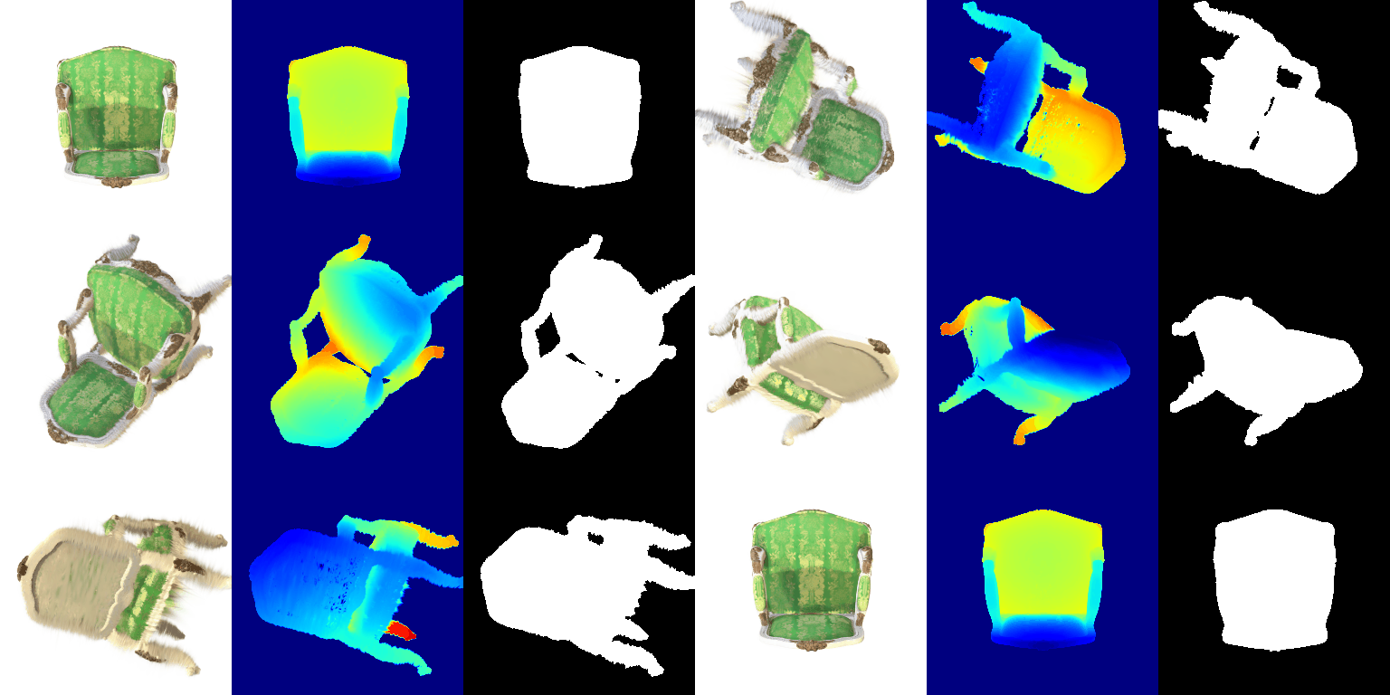
32 views; RGB, depth, silhouette from left to right.
Rotation convention: PyTorch3D's row-vector convention implies W = R.T in the covariance formula. Following the instructor's forum guidance, I use W = R to match the supplied tests. Comparing both conventions showed reduced stretching with R.T at steep angles.
10,000 isotropic Gaussians initialized from the supplied point cloud; Adam with L1 RGB loss.
| Parameter | Learning rate |
|---|---|
| Means | 0.00016 |
| Scales | 0.005 |
| Colors | 0.0025 |
| Opacities | 0.05 |
| Setting / metric | Value |
|---|---|
| Iterations | 1,000 |
| Resolution / seed | 160 × 90 / 1 |
| Held-out PSNR | 29.416 dB |
| Held-out SSIM | 0.9399 |
Top: predictions. Bottom: ground truth.
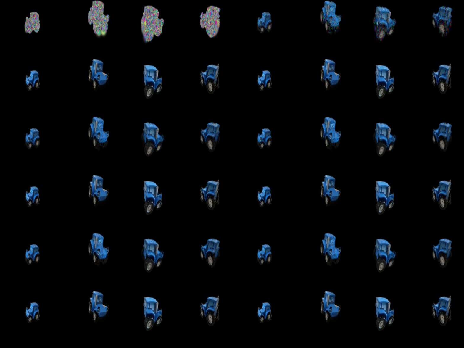
197 training views; the metrics above use five separate held-out views.

The pretrained coefficients are evaluated using all 16 SH basis functions through degree 3.
| Degree-0 color | Degree-3 spherical harmonics |
|---|---|
|
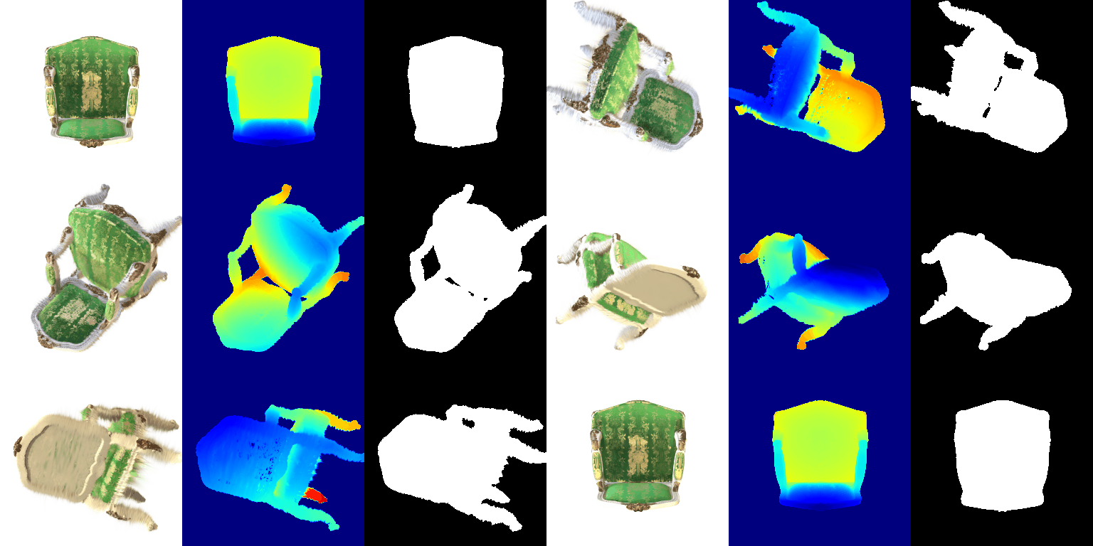 |
Each RGB pair uses the same camera: DC only on the left, full SH on the right.

SH produces darker green upholstery and stronger contrast in the fabric pattern.

SH changes local brightness on the fabric and wood. Both retain stretching associated with the covariance convention discussed in Section 5.

SH gives a less washed-out green surface and a more distinct pattern; the silhouette stays the same.