

Everything was run on an RTX 5090. Part A is in nerf/ and Part B in GS/.
Pixel centres are mapped to NDC in [-1, 1], placed on the z = 1 plane and unprojected to world space with
camera.unproject_points. Every ray starts at the camera centre and points through its unprojected
pixel, normalised to unit length.
The stratified sampler places 64 points uniformly between the near and far depth (0 and 5) on every ray,
p = o + t d. The point cloud below is all sample points of the first camera's rays.

For each sample, alpha is 1 - exp(-σ Δt) and the transmittance is the cumulative product of
1 - alpha over the earlier samples (1 for the first sample). The weights are
T * alpha, the colour is the weighted sum of the sample colours, and the depth is the weighted
sum of the sample distances. The depth map is normalised by its maximum.


get_random_pixels_from_image shuffles the full pixel grid with torch.randperm and
keeps the first 4096 pixels, so every iteration trains on a random subset of rays without repeats.
The loss is the mean squared error between the rendered colours and the ground-truth colours at the sampled pixels. After 1000 epochs:
| x | y | z | |
|---|---|---|---|
| Box center | 0.25 | 0.25 | 0.00 |
| Box side lengths | 2.01 | 1.50 | 1.50 |

Each sample point is encoded with 6 harmonic frequencies (39-D with the raw xyz) and passed through a 6-layer MLP with 128 hidden units and ReLU, where the encoding is concatenated again at layer 3 as a skip connection. Two heads read the 128-D feature: a linear layer with ReLU for the density, and a 128 → 64 → 3 MLP with a sigmoid for the colour. The model has no view dependence here. I trained it with the MSE loss for 250 epochs on the 128x128 lego images, with 1024 rays per iteration, 128 samples per ray between depth 2 and 6, and learning rate 5e-4 decayed by 0.8 every 50 epochs.

The viewing direction of each ray is copied to all of its sample points, encoded with 2 harmonic
frequencies (15-D) and concatenated to the 128-D feature, but only after the density has been computed.
The density therefore depends on position only and only the small colour head sees the direction. A flag
view_dependence in the config turns this on, so the lego model from Q3 is unchanged. I trained
on the materials scene at 128x128 with and without view dependence, and at 400x400 with it
(nerf_materials.yaml and nerf_materials_highres.yaml, 250 epochs each).


PSNR on 20 training views and 20 held-out test views (epoch-200 checkpoints):
| Model | Train PSNR | Test PSNR | Gap |
|---|---|---|---|
| No view dependence, 128 | 23.29 | 21.25 | 2.04 |
| View dependence, 128 | 23.66 | 21.40 | 2.26 |
| View dependence, 400 | 24.39 | 21.87 | 2.52 |
With view dependence the highlights on the metallic spheres move across the surface as the camera orbits, while without it the spheres look flat and matte, since a single colour per point has to average the highlight over all views. Both train and test PSNR improve, but the train improvement is larger and the gap between them grows. The extra freedom lets the network explain parts of the training images with the viewing direction instead of the geometry, which is a form of overfitting. With only 100 training views, the directions in between are interpolated by the colour head, so too much view dependence gives worse novel views. That is why I followed the NeRF paper: the direction enters only after the density (the geometry has to be consistent across all views), it uses fewer frequencies than the position (smooth changes with angle) and it goes through a small head. More view dependence fits shiny materials better at the cost of generalisation.
The 3D covariance is R S Sᵀ Rᵀ with R from the quaternion and S the diagonal of scales (just
s² I for isotropic Gaussians, whose quaternions are never used). It is projected to 2D with
J W Σ Wᵀ Jᵀ, using the camera rotation as W and the perspective Jacobian J, and the means are
projected with transform_points_screen. Gaussians are sorted by view-space depth and those with
depth below 0 are removed. Alpha is opacity * exp(power), the transmittance is the cumulative
product of 1 - alpha, and the colour, depth and mask are the sums of colour, depth and 1 weighted
by alpha * T. All 4 unit tests pass.

The 10,000 isotropic Gaussians are initialised from the truck point cloud. I trained them with an L1 loss for 1000 iterations using these learning rates (Adam):
| Parameter | Learning rate |
|---|---|
| Opacities (pre-sigmoid) | 0.05 |
| Scales (log) | 0.005 |
| Colours | 0.01 |
| Means | 0.001 |
The opacities start at 8 before the sigmoid, so they need a large rate to change at all, while the means need a small one so the Gaussians don't drift off the truck. I also tried means at 0.0005 and 0.002 and colours at 0.02 and 0.05, which were all slightly worse.
PSNR = 29.981, SSIM = 0.942

Training progress (top: renders, bottom: ground truth).

Final renders of the training views.
The chair Gaussians store degree-3 spherical harmonics, 16 coefficients per colour channel. For each Gaussian I compute the unit direction from the camera centre to its mean, evaluate the 16 SH basis functions at that direction and take their weighted sum with the coefficients, plus 0.5 and clamped at 0. With only the first (DC) coefficient this gives exactly the colours used in 5.5.

Side-by-side RGB renders of the same frame (left: DC only, right: spherical harmonics):

Frame 3: with SH the fabric is a deeper green with darker shading in the folds and the gold trim looks brighter and more metallic. With DC only the chair looks flat and washed out, like matte paint.

Frame 12: the same effect on the back, with more contrast in the fabric pattern and highlights on the carved wood. This is the largest difference of the three frames (mean 6.1 out of 255).

Frame 20: the underside is matte beige and the two renders are almost identical (mean difference 1.8). Its colour hardly depends on the viewing direction, so the higher SH terms add almost nothing there.
Baseline. The same setup as Q6 (isotropic Gaussians, the Q6 learning rates, L1 loss, 1000 iterations) with 10,000 Gaussians at random init on the materials scene: PSNR = 18.293, SSIM = 0.694.

Baseline training progress.
The random init puts all Gaussians in a ball of standard deviation 0.2 around the origin, while the objects spread over roughly ±1.5. With a means learning rate of 0.001 most Gaussians never reach the outer objects, which stay blurry smears. Training twice as long barely helps (19.00).
Improved. PSNR = 22.944, SSIM = 0.851 after 2000 iterations. The changes are:
0.8 * L1 + 0.2 * (1 - SSIM) as in the 3DGS paper, with a differentiable
SSIM (11x11 Gaussian window). It rewards local structure such as edges and texture, not only per-pixel
colour.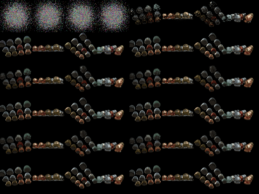
Improved training progress.


Experiments, each adding one change and trained for 2000 iterations (single runs, so differences under about 0.5 dB are within run-to-run noise from the random init):
| Setting | PSNR | SSIM |
|---|---|---|
| Baseline setup, 2000 iterations | 19.00 | 0.709 |
| + wider init (std 0.8) | 22.67 | 0.828 |
| + means lr 0.005 and lr decay | 22.68 | 0.831 |
| + SSIM loss | 22.72 | 0.841 |
| + anisotropic | 22.76 | 0.843 |
| + init std 0.5 instead of 0.8 (final) | 22.99 | 0.854 |
| final, init std 1.2 instead | 22.25 | 0.817 |
| final with 4.5x larger initial scales | 21.67 | 0.803 |
| final with 15,000 Gaussians | 22.82 | 0.847 |
Larger initial scales made the Gaussians overlap and blur the result, and 15,000 Gaussians gave a similar score for about 50% more memory and time, so I kept 10,000. The remaining errors are mostly the dark caps of the objects, which blend into the black background, and grainy edges where the Gaussians are still small.