Single View to 3D
16-825 Learning for 3D: Assignment 2
Author: Benny Zhu (haozhenz)
Date: October 2026


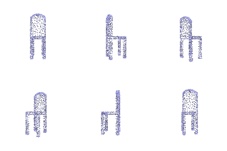

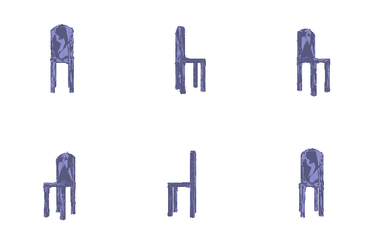
2. Reconstructing 3D from Single View (80 Points)
2.1 Image to Voxel Grid (20 points)
python train_model.py --type vox --max_iter 5000 --num_workers 8 --save_freq 500
python eval_model.py --type 'vox' --load_checkpoint
| Example | Input RGB | Predicted Voxel Grid | Ground Truth Mesh |
|---|---|---|---|
| 1 |  |
 |
 |
| 2 |  |
 |
 |
| 3 |  |
 |
 |
F1@0.05 = 0.38
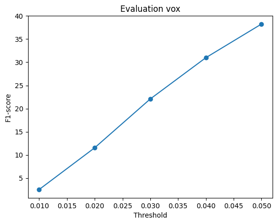
Due to limited computational resources and time, the maximum number of iterations was capped at 5,000; under this budget, I did not get satisfactory performance with voxel.
2.2 Image to Point Cloud (20 points)
python train_model.py --type point --max_iter 5000 --num_workers 8 --save_freq 500
python eval_model.py --type 'point' --load_checkpoint
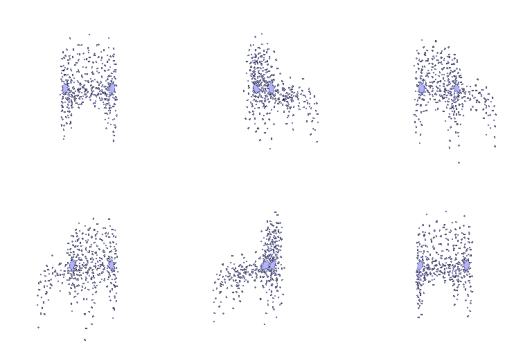
| Example | Input RGB | Predicted Point Cloud | Ground Truth Point Cloud |
|---|---|---|---|
| 1 |  |
 |
 |
| 2 |  |
 |
 |
| 3 |  |
 |
 |
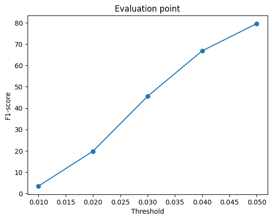
F1@0.05 = 0.8
2.3 Image to Mesh (20 points)
python train_model.py --type mesh --max_iter 5000 --num_workers 8 --save_freq 500
python eval_model.py --type 'mesh' --load_checkpoint
| Example | Input RGB | Predicted Mesh | Ground Truth Mesh |
|---|---|---|---|
| 1 |  |
 |
 |
| 2 |  |
 |
 |
| 3 |  |
 |
 |
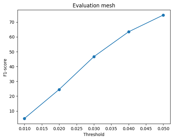
F1@0.05 = 0.78
Due to limited computational resources and time, the maximum number of iterations was capped at 5,000; under this budget, I did not get satisfactory performance with mesh.
Voxel vs. Point Cloud vs. Mesh Comparison
| Representation | F1@0.05 |
|---|---|
| Voxel Grid | 38% |
| Point Cloud | 80% |
| Mesh | 78% |
From the score curve above, we observe that the point cloud model achieves the best F1 score, followed by the mesh model, with the voxel grid model performing the worst. This ordering can be explained by how much freedom each representation gives the model to fit the target geometry. The point cloud model is the least constrained. Each point's position is predicted independently, so the network can move points wherever they best match the target shape. The mesh model is more constrained, since vertices are connected by faces into a fixed topology. The model must learn vertex offsets that not only approximate the target shape but also keep the resulting surface smooth and non-self-intersecting, which is a harder optimization problem than freely placing independent points. The voxel grid model is the most constrained of the three. It predicts occupancy over a fixed, low-resolution 32³ grid, so any geometry finer than the voxel size simply cannot be represented, regardless of how well the network is trained.
2.4 Analyse Effects of Hyperparameter Variations (10 points)
Hyperparameter: w_smooth
| Setting | F1@0.05 | Example Prediction |
|---|---|---|
w_smooth = 0.1 |
78% | |
w_smooth = 1.0 |
74% |  |
w_smooth directly controls the trade-off between two competing objectives when fitting a mesh: loss_reg pulls vertices toward matching the target geometry as closely as possible, while loss_smooth pulls each vertex toward the average position of its neighbors, discouraging sharp, noisy surfaces.
Increasing w_smooth from 0.1 to 1.0 noticeably reduces the needle-like spikes covering the surface. The mesh looks more blocky rather than coated in thin jagged protrusions. That said, the stronger smoothing weight does not fully eliminate surface noise. Both meshes still show torn, irregular edges around the legs and a rough silhouette overall, suggesting the Laplacian term alone isn't enough to pull the ico-sphere topology into a clean chair shape at this training budget. The chamfer term still dominates locally, so vertices get pulled toward the target surface in a way that creates sharp local folds even while the broader regularization pushes neighboring vertices toward agreement.
2.5 Interpret Your Model (10 points)
| Example 1 | Example 2 | Example 3 |
|---|---|---|
 |
 |
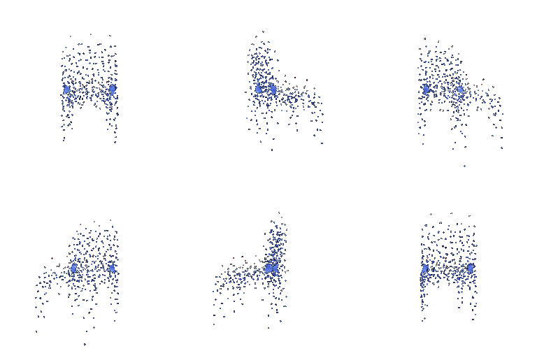 |
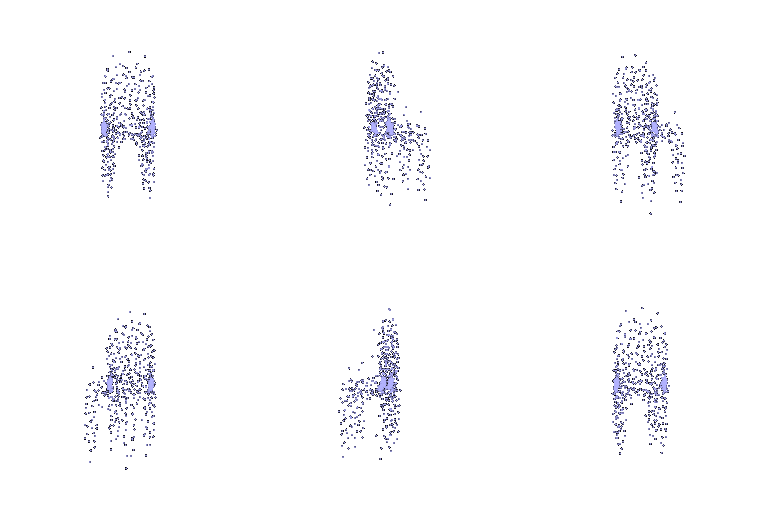
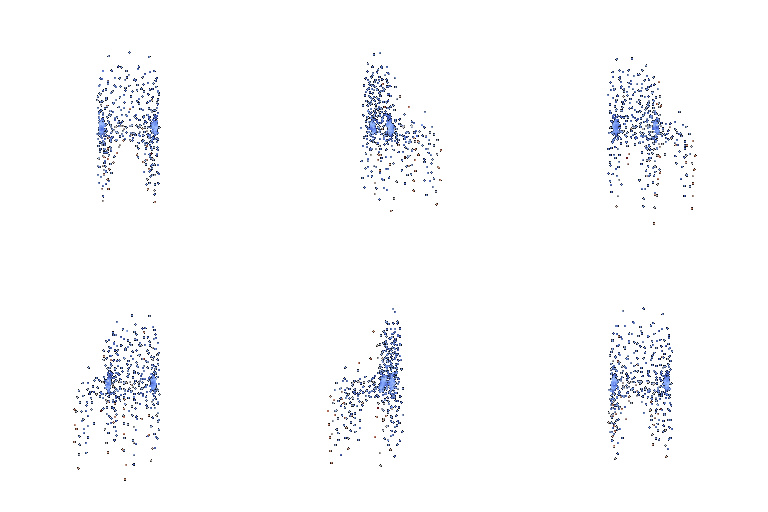
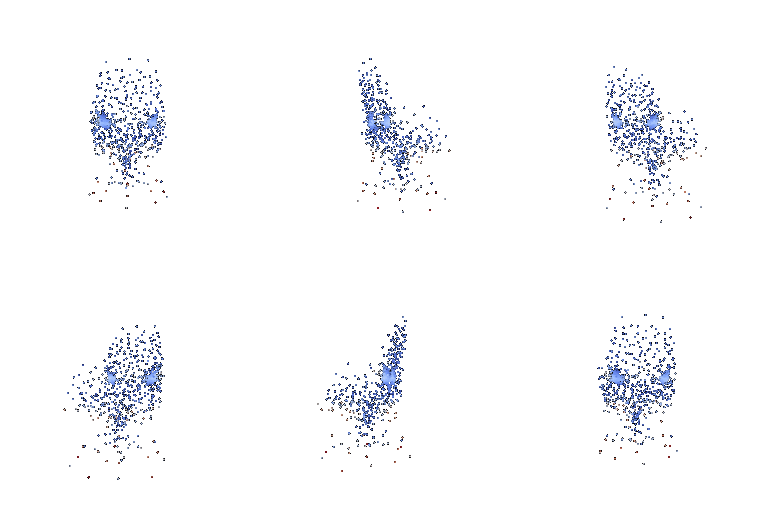
Per-vertex error heatmap: For each predicted point or vertex, we compute its Euclidean distance to the nearest point in the ground-truth point cloud, then map that distance to a color on a blue→red scale: blue = prediction is close to the true surface at that location, red = prediction is far off.
Across all three test samples, the model consistently performs well on large, continuous regions of the shape, but systematically struggles on thin, elongated structures, which matches the intuition discussed when comparing voxel, mesh and point cloud representation in Q2.3.
3. Exploring Other Architectures / Datasets (10 Points)
3.2 Parametric Network (10 points)
python train_model.py --type parametric --max_iter 5000 --num_workers 8 --save_freq 500
python eval_model.py --type 'parametric' --load_checkpoint
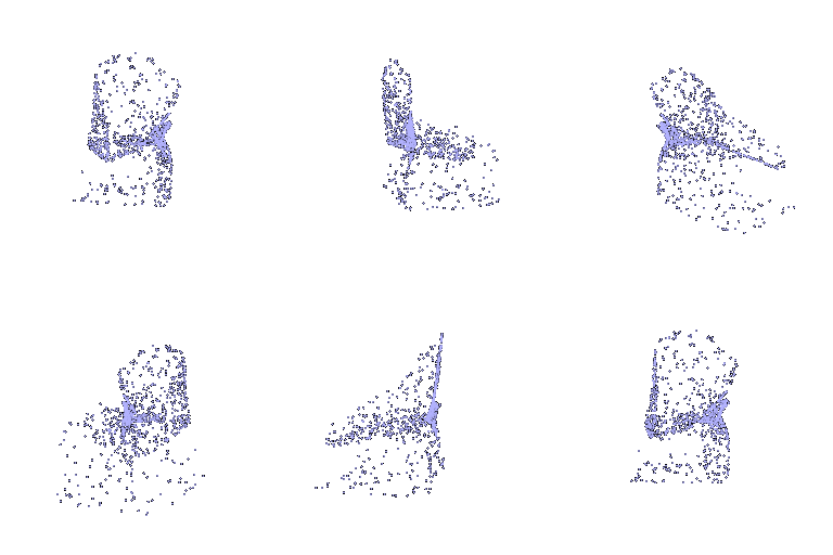
| Example | Input RGB | Prediction | Ground Truth Mesh |
|---|---|---|---|
| 1 |  |
 |
 |
| 2 |  |
 |
 |
| 3 |  |
 |
 |
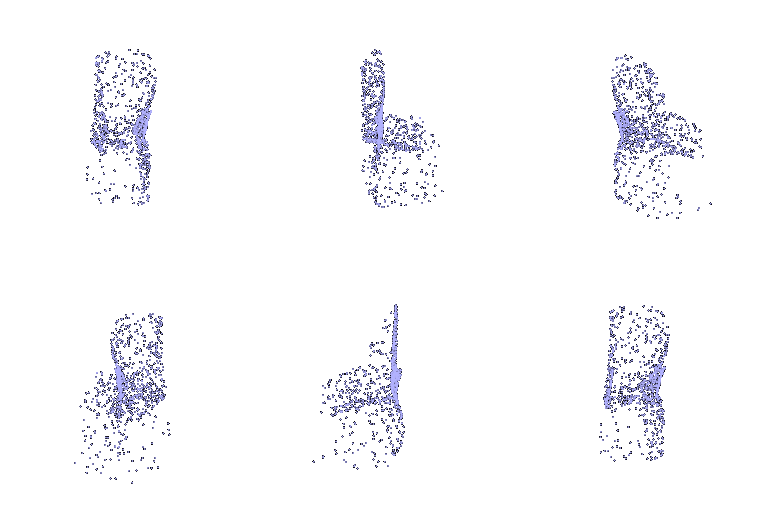
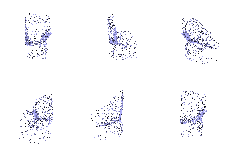
F1@0.05 =65%
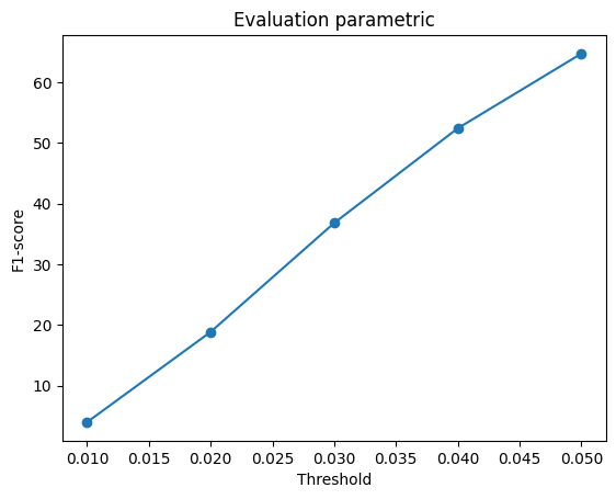
The parametric architecture is, in principle, less prone to mode collapse, since its explicit 2D coordinate input gives the network a stronger structural prior that naturally spreads the predicted points apart. The trade-off, however, is slower convergence and lower accuracy under the same training budget. With a smaller per-point decoder and a noisier training signal, it simply has more to learn from the same number of iterations. Widening the parametric decoder's hidden layers or training it for longer would likely narrow this gap, but as it stands, this result shows that a more "elegant" architecture does not automatically translate into a higher score under a fixed training budget.